Mark W. Spong - Robot Modeling and Control

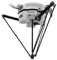
Figure 1.17 The ABB IRB360 parallel robot. Parallel robots generally have higher structural rigidity than serial link robots. (Photo courtesy of ABB.)

The present textbook is divided into four parts. The first three parts are devoted to the study of manipulator arms. The final part treats the control of underactuated and mobile robots.

We can use the simple example below to illustrate some of the major issues involved in the study of manipulator arms and to preview the topics covered. A typical application involving an industrial manipulator is shown in Figure 1.18. The manipulator is shown with a grinding tool that it must use to remove a certain amount of metal from a surface. Suppose we wish to move the manipulator from its homeposition to position A , from which point the robot is to follow the contour of the surface S to the point B , at constant velocity, while maintaining a prescribed force F normal to the surface. In so doing the robot will cut or grind the surface according to a predetermined specification. To accomplish this and even more general tasks, we must solve a number of problems. Below we give examples of these problems, all of which will be treated in more detail in the text.

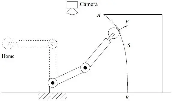
Figure 1.18 Two-link planar robot example. Each chapter of the text discusses a fundamental concept applicable to the task shown.

The first problem encountered is to describe both the position of the tool and the locations A and B (and most likely the entire surface S ) with respect to a common coordinate system. In Chapter 2we describe representations of coordinate systems and transformations among various coordinate systems. We describe several ways to represent rotations and rotational transformations and we introduce so-called homogeneous transformations, which combine position and orientation into a single matrix representation.

Typically, the manipulator will be able to sense its own position in some manner using internal sensors (position encoders located at joints 1 and 2) that can measure directly the joint angles θ 1and θ 2. We also need therefore to express the positions A and B in terms of these joint angles. This leads to the forward kinematics problemstudied in Chapter 3, which is to determine the position and orientation of the end effector or tool in terms of the joint variables.

It is customary to establish a fixed coordinate system, called the worldor baseframe to which all objects including the manipulator are referenced. In this case we establish the base coordinate frame o 0 x 0 y 0at the base of the robot, as shown in Figure 1.19. The coordinates ( x , y ) of the tool are expressed in this coordinate frame as

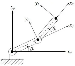
Figure 1.19 Coordinate frames attached to the links of a two-link planar robot. Each coordinate frame moves as the corresponding link moves. The mathematical description of the robot motion is thus reduced to a mathematical description of moving coordinate frames.

(1.1)

(1.2)

in which a 1and a 2are the lengths of the two links, respectively. Also the orientation of the tool framerelative to the base frame is given by the direction cosines of the x 2and y 2axes relative to the x 0and y 0axes, that is,

(1.3)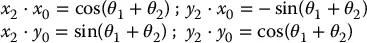

which we may combine into a rotation matrix

(1.4)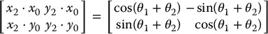

Equations ( 1.1), ( 1.2), and ( 1.4) are called the forward kinematic equationsfor this arm. For a six-DOF robot these equations are quite complex and cannot be written down as easily as for the two-link manipulator. The general procedure that we discuss in Chapter 3establishes coordinate frames at each joint and allows one to transform systematically among these frames using matrix transformations. The procedure that we use is referred to as the Denavit–Hartenbergconvention. We then use homogeneous coordinatesand homogeneous transformations, developed in Chapter 2, to simplify the transformation among coordinate frames.

To follow a contour at constant velocity, or at any prescribed velocity, we must know the relationship between the tool velocity and the joint velocities. In this case we can differentiate Equations ( 1.1) and ( 1.2) to obtain

(1.5)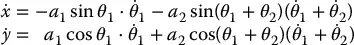

Using the vector notation and , we may write these equations as

(1.6)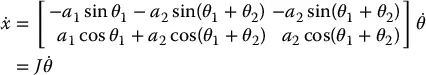

The matrix J defined by Equation ( 1.6) is called the Jacobianof the manipulator and is a fundamental object to determine for any manipulator. In Chapter 4we present a systematic procedure for deriving the manipulator Jacobian.

The determination of the joint velocities from the end-effector velocities is conceptually simple since the velocity relationship is linear. Thus, the joint velocities are found from the end-effector velocities via the inverse Jacobian

(1.7)

where J − 1is given by

The determinant of the Jacobian in Equation ( 1.6) is equal to a 1 a 2sin θ 2. Therefore, this Jacobian does not have an inverse when θ 2= 0 or θ 2= π, in which case the manipulator is said to be in a singular configuration, such as shown in Figure 1.20for θ 2= 0. The determination of such singular configurations is important for several reasons. At singular configurations there are infinitesimal motions that are unachievable; that is, the manipulator end effector cannot move in certain directions. In the above example the end effector cannot move in the positive x 2direction when θ 2= 0. Singular configurations are also related to the nonuniqueness of solutions of the inverse kinematics. For example, for a given end-effector position of the two-link planar manipulator, there are in general two possible solutions to the inverse kinematics. Note that a singular configuration separates these two solutions in the sense that the manipulator cannot go from one to the other without passing through a singularity. For many applications it is important to plan manipulator motions in such a way that singular configurations are avoided.