A. Gouveia Oliveira - Biostatistics Decoded

It is an easy mathematical exercise to demonstrate that dividing the sum of squares by n − 1 instead of n provides an adequate correction of that bias. However, the same thing can be shown by the small experiment illustrated in Figures 1.12and 1.13.

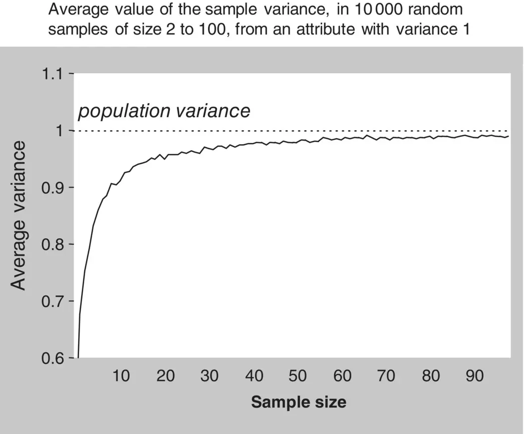
Figure 1.12 The n divisor of the sum of squares.

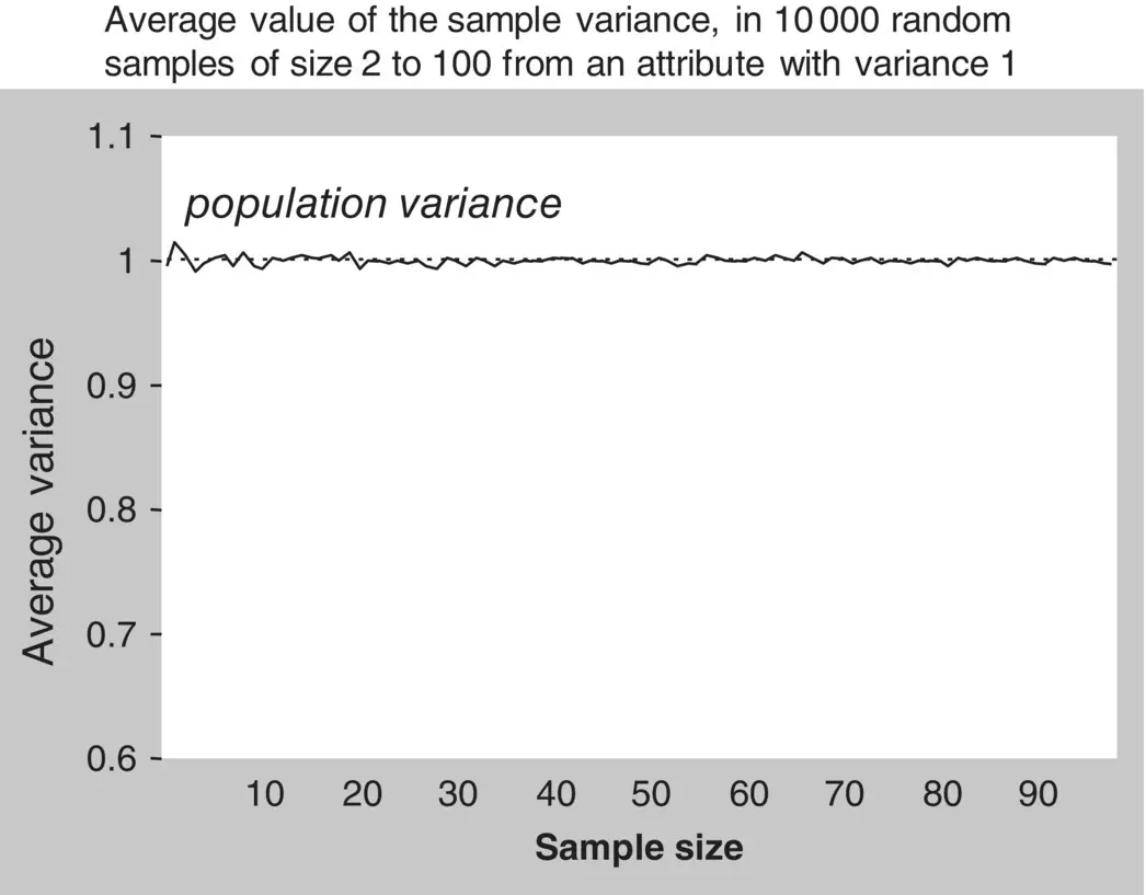
Figure 1.13 The n − 1 divisor of the sum of squares.

Using a computer’s random number generator, we obtained random samples of a variable with variance equal to 1. This is the population variance of that variable. Starting with samples of size 2, we obtained 10 000 random samples and computed their sample variances using the n divisor. Next, we computed the average of those 10 000 sample variances and retained the result. We then repeated the procedure with samples of size 3, 4, 5, and so on up to 100.

The plot of the averaged value of sample variances against sample size is represented by the solid line in Figure 1.12. It can clearly be seen that, regardless of the sample size, the variance computed with the n divisor is on average less than the population variance, and the deviation from the true variance increases as the sample size decreases.

Now let us repeat the procedure, exactly as before, but this time using the n − 1 divisor. The plot of the average sample variance against sample size is shown in Figure 1.13. The solid line is now exactly over 1, the value of the population variance, for all sample sizes.

This experiment clearly illustrates that, contrary to the sample variance using the n divisor, the sample variance using the n − 1 divisor is an unbiased estimator of the population variance.

Degrees of freedomis a central notion in statistics that applies to all problems of estimation of quantities in populations from the observations made on samples. The number of degrees of freedom is the number of values in the calculation of a quantity that are free to vary. The general rule for finding the number of degrees of freedom for any statistic that estimates a quantity in the population is to count the number of independent values used in the calculation minus the number of population quantities that were replaced by sample quantities during the calculation.

In the calculation of the variance, instead of summing the squared differences of each value to the population mean , we summed the squared differences to the sample mean . Therefore, we replaced a population parameter by a sample parameter and, because of that, we lose one degree of freedom. Therefore, the number of degrees of freedom of a sample variance is n − 1.

As a binary variable is a numeric variable, in addition to calculating a mean, which is called a proportion in binary variables, we can also calculate a variance. The computation is the same as for interval variables: the differences of each observation from the mean are squared, then summed up and divided by the number of observations. With binary l variables there is no need to correct the denominator and the sum of squares is divided by n .

An easier method of calculating the variance of a binary attribute is simply by multiplying the proportion with the attribute by the proportion without the attribute. If we represent the proportion with the attribute by p , then the variance will be p (1 − p ). For example, if in a sample of 110 people there were 9 with diabetes, the proportion with diabetes is 9/110 = 0.082 and the variance of diabetes is 0.082 × (1 − 0.082) = 0.075. Therefore, there is a fixed relationship between a proportion and its variance, with the variance increasing for proportions between 0 and 0.5 and decreasing thereafter, as shown in Figure 1.14.

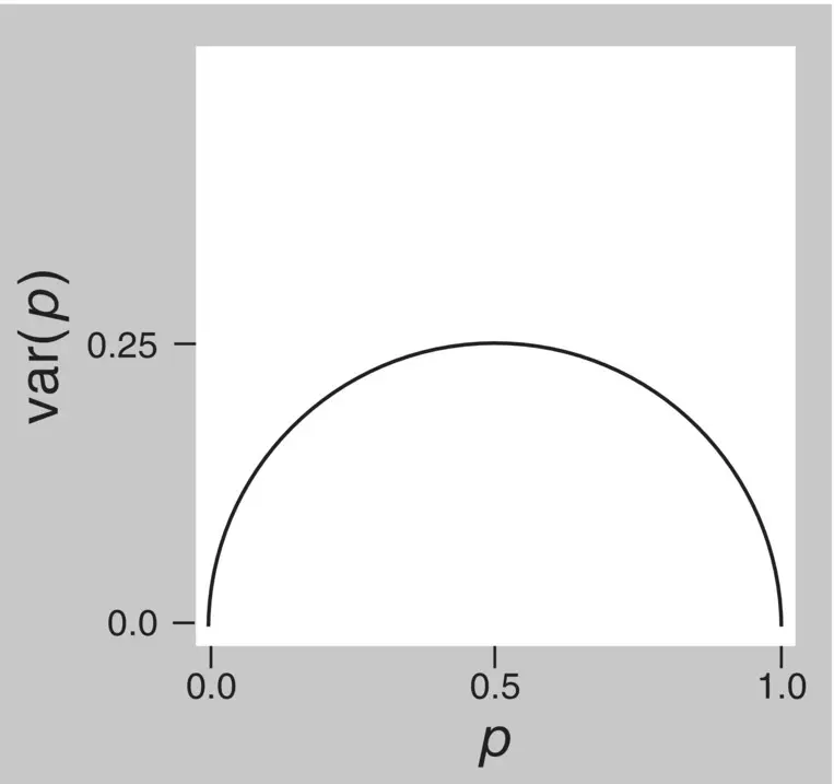
Figure 1.14 Relationship between a proportion and its variance.

Means and variances have some interesting properties that deserve mention. Knowledge of some of these properties will be very helpful when analyzing the data, and will be required several times in the following sections. Regardless, they are all intuitive and easy to understand.

With a computer, we generated random numbers between 0 and 1, representing observations from a continuous attribute with uniform distribution, which we will call variable A . This attribute is called a random variablebecause it can take any value from a set of possible distinct values, each with a given probability. In this case, variable A can take any value from the set of real numbers between 0 and 1, all with equal probability. Hence the probability distributionof variable A is called the uniform distribution.

A second variable, called variable B , with uniform distribution but with values between 0 and 2, was also generated. The distributions of the observed values of those variables are shown in the graphs of Figure 1.15. That type of graph is called a histogram, the name given to the graph of a continuous variable where the values are grouped in binsthat are plotted adjacent to each other. Let us now see what happens to the mean and variance when we perform arithmetic operations on a random variable.

When a constant amount is added to, or subtracted from, the values of a random variable, the mean will, respectively, increase or decrease by that amount but the variance will not change. This is illustrated in Figure 1.16(left graph), which shows the distribution of variable A plus 2. This result is obvious, because, as all values are increased (or decreased) by the same amount, the mean will also increase (or decrease) by that amount and the distance of each value from the mean will thus remain the same, keeping the variance unchanged.

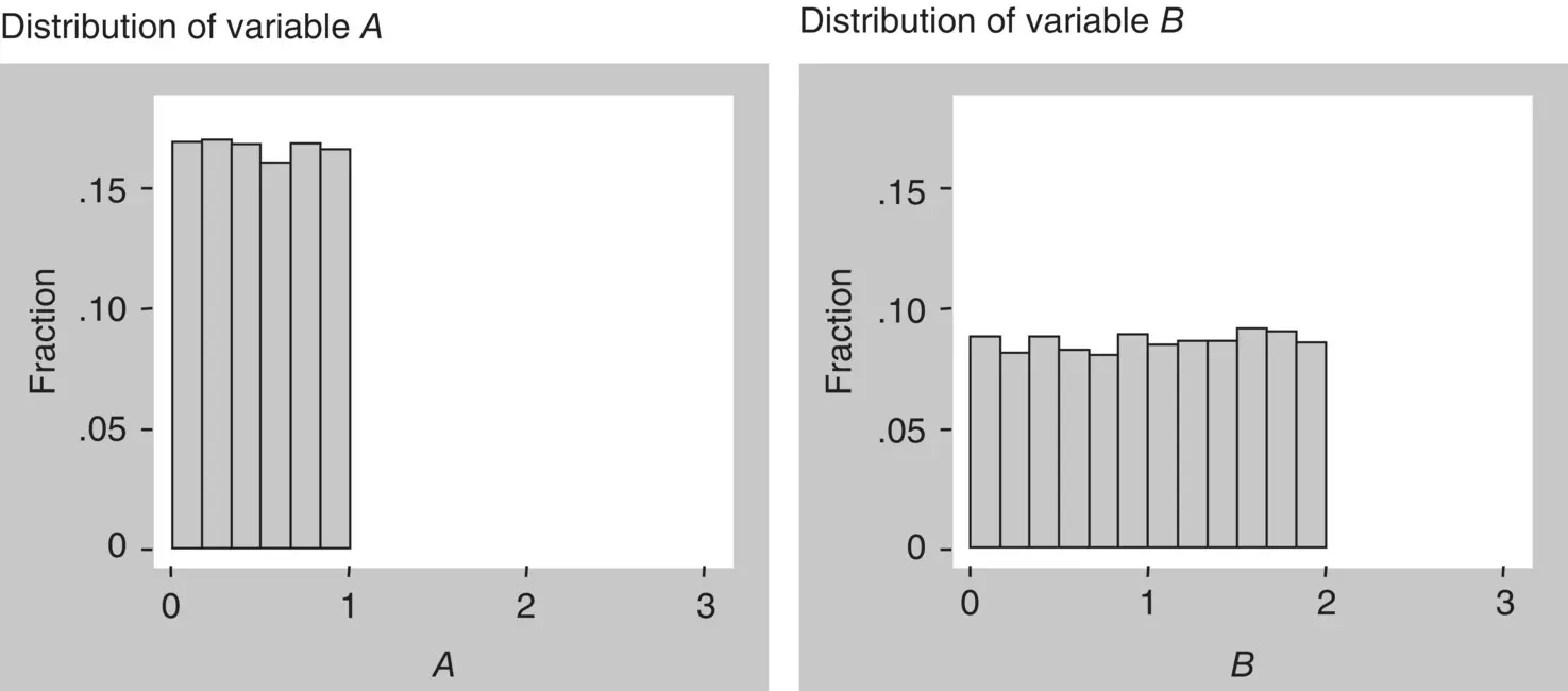
Figure 1.15 Two random variables with uniform distribution.

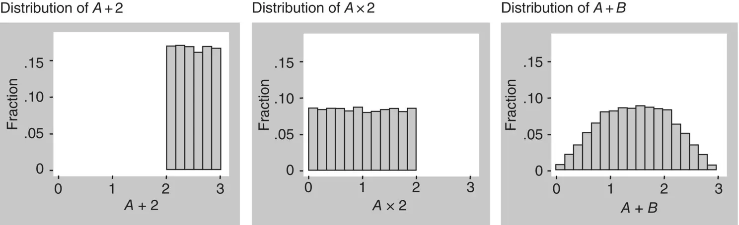
Figure 1.16 Properties of means and variances.

When a constant amount multiplies, or divides, the values of a random variable, the mean will be, respectively, multiplied or divided by that amount, and the variance will be, respectively, multiplied or divided by the square of that amount. Therefore, the standard deviation will be multiplied or divided by the same amount. Figure 1.16(middle graph), shows the distribution of A multiplied by 2. As an example, consider the attribute height with mean 1.7 m and standard deviation 0.6 m. If we want to convert the height to centimeters, we multiply all values by 100. Now the mean will of course be 170 cm and the standard deviation 60 cm. Thus, the mean was multiplied by 100 and the standard deviation also by 100 (and, therefore, the variance was multiplied by 100 2).