A. Gouveia Oliveira - Biostatistics Decoded

However, we still have the problem of having to deal with two values, which is certainly not as practical and easy to remember, and to reason with, as if we had just one value. One way around this could be to use the difference between the upper quartile and the lower quartile to describe the dispersion. This is called the interquartile range, but the interpretation of this value is not straightforward: it is not amenable to mathematical treatment and therefore it is not a very popular measure, except perhaps in epidemiology.

So what are we looking for in a measure of dispersion? The ideal measure should have the following properties: unicity, that is, it should be a single value; stability, that is, it should not change much if more observations are added; interpretability, that is, its value should meaningful and easy to understand.

Let us now consider other measures of dispersion. Another possible measure could be the average of the deviations of all individual values about the mean or, in other words, the average of the differences between each value and the mean of the distribution. This would be an interesting measure, being both a single value and easy to interpret, since it is an average. Unfortunately, it would not work because the differences from the mean in those values smaller than the mean are positive, and the differences in those values greater than the mean are negative. The result, if the values are symmetrically distributed about the mean, will always be close to zero regardless of the magnitude of the dispersion.

Actually, what we want is the average of the size of the differences between the individual values and the mean. We do not really care about the direction (or sign) of those differences. Therefore, we could use instead the average of the absolute value of the differences between each value and the mean. This quantity is called the absolute mean deviation. It satisfies the desired properties of a summary measure: single value, stability, and interpretability. The mean deviation is easy to interpret because it is an average, and people are used to dealing with averages. If we were told that the mean of some patient attribute is 256 mmol/l and the mean deviation is 32 mmol/l, we could immediately figure out that about half the values were in the interval 224–288 mmol/l, that is, 256 − 32 to 256 + 32.

There is a small problem, however. The mean deviation uses absolute values, and absolute values are quantities that are difficult to manipulate mathematically. Actually, they pose so many problems that it is standard mathematical practice to square a value when one wants the sign removed. Let us apply that method to the mean deviation. Instead of using the absolute value of the differences about the mean, let us square those differences and average the results. We will get a quantity that is also a measure of dispersion. This quantity is called the variance. The way to compute the variance is, therefore, first to find the mean, then subtract each value from the mean, square the result, and add all those values. The resulting quantity is called the sum of squares about the mean, or just the sum of squares. Finally, we divide the sum of squares by the number of observations to get the variance.

Because the differences are squared, the variance is also expressed as a square of the attribute’s units, something strange like mmol 2/l 2. This is not a problem when we use the variance for calculations, but when in presentations it would be rather odd to report squared units. To put things right we have to convert these awkward units into the original units by taking the square root of the variance. This new result is also a measure of dispersion and is called the standard deviation.

As a measure of dispersion, the standard deviation is single valued and stable, but what can be said about its interpretability? Let us see: the standard deviation is the square root of the average of the squared differences between individual values and the mean. It is not easy to understand what this quantity really represents. However, the standard deviation is the most popular of all measures of dispersion. Why is that?

One important reason is that the standard deviation has a large number of interesting mathematical properties. The other important reason is that, actually, the standard deviation has a straightforward interpretation, very much along the lines given earlier to the value of the mean deviation. However, we will go into that a little later in the book.

A final remark about the variance. Although the variance is an average, the total sum of squares is divided not by the number of observations as an average should be, but by the number of observations minus 1, that is, by n − 1.

It does no harm if we use symbols to explain the calculations. The formula for the calculation of the variance of an attribute x is

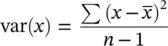
where ∑ (capital “S” in the Greek alphabet) stands for summation and represents the mean of attribute x . So, the expression reads “sum all the squared differences of each value to the overall mean and then divide by the sample size.”

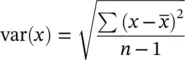
Naturally, the formula for the standard deviation is

The reason why we use the n − 1 divisor instead of the n divisor for the sum of squares when we calculate the variance and the standard deviation is because, when we present those quantities, we are implicitly trying to give an estimate of their value in the population. Now, since we use the data from our sample to calculate the variance, the resulting value will always be smaller than the value of the variance in the population. We say that our result is biasedtoward a smaller value. What is the explanation for that bias?

Remember that the variance is the average of the squared differences between individual values and the mean. If we calculated the variance by subtracting the individual values from the true mean (the population mean), the result would be unbiased. This is not what we do, though. We subtract the individual values from the sample mean. Since the sample mean is the quantity closest to all the values in the dataset, individual values are more likely to be closer to the sample mean than to the population mean. Therefore, the value of the sample variancetends to be smaller than the value of the population variance. The variance is a good measure of dispersion of the values observed in a sample, but is biasedas a measure of dispersion of the values in the population from which the sample was taken. However, this bias is easily corrected if the sum of squares is divided by the number of observations minus 1.

This book is written at two levels of depth: the main text is strictly non‐mathematical and directed to those readers who just want to know the rationale of biostatistical concepts and methods in order to be able to understand and critically evaluate the scientific literature; the text boxes intermingled in the main text present the mathematical formulae and the description of the procedures, supported by working examples, of every statistical calculation and test presented in the main text. The former readers may skip the text boxes without loss of continuity in the presentation of the topics.