A. Gouveia Oliveira - Biostatistics Decoded

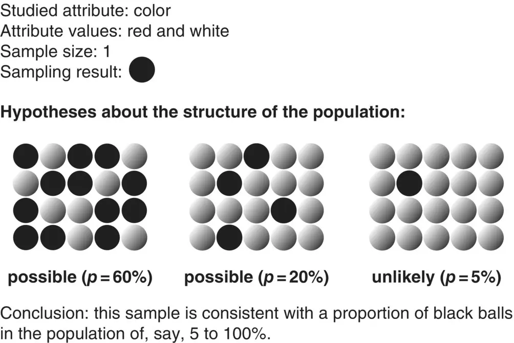
Figure 1.8 Inference with binary attributes.

Suppose now that we decide to take a random sample of 60 balls, and that we have 24 black balls and 36 white balls ( Figure 1.9). The proportion of black balls in the sample is, therefore, 40%. What can we say about the proportion of black balls in the population? Well, we can say that if the proportion is below, say, 25%, there should not be so many black balls in a sample of 60. Conversely, we can also say that if the proportion is above, say, 55%, there should be more black balls in the sample. Therefore, we would be confident in concluding that the proportion of black balls in the swimming pool must be somewhere between 25 and 55%. This is a more interesting result than the previous one because it has more precision; that is, the range of possibilities is narrower than before. If we need more precision, all we have to do is increase the sample size.

Let us return to the situation of a sample size of one and suppose that we want to estimate another characteristic of the balls in the population, for example, the average weight. This characteristic, or attribute, has an important difference from the color attribute, because weight can take many different values, not just two.

Let us see if we can apply the same reasoning in the case of attributes taking many different values. To do so, we take a ball at random and measure its weight. Let us say that we get a weight of 60 g. What can we conclude about the average weight in the population? Now the answer is not so simple. If we knew that the balls were all about the same weight, we could say that the average weight in the population should be a value between, say, 50 and 70 g. If it were below or above those limits, it would be unlikely that a ball sampled at random would weigh 60 g.

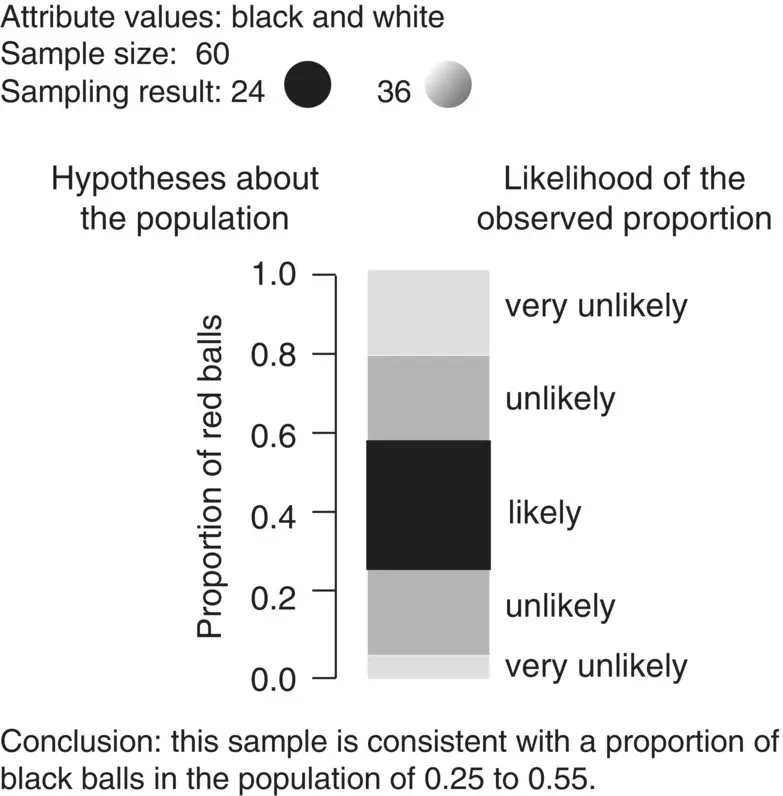
Figure 1.9 Inference with interval attributes I.

However, if we knew that the balls varied greatly in weight, we would say that the average weight in the population should be a value between, say, 40 and 80 g ( Figure 1.10). The problem here, because now we are studying an attribute that may take many values, is that to make inferences about the population we also need information about the amount of variation of that attribute in the population. It thus appears that this approach does not work well in this extreme situation. Or does it?

Suppose we take a second random observation and now have a sample of two. The second ball weighs 58 g, and so we are compelled to believe that balls in this population are relatively homogeneous regarding weight. In this case, we could say that we were quite confident that the average weight of balls in the population was between 50 and 70 g. If the average weight were under 50 g, it would be unlikely that we would have two balls with 58 and 60 g in the sample; and similarly if the average weight were above 70 g. So this approach works properly with a sample size of two, but is this situation extreme? Yes it is, because in this case we need to estimate not one but two characteristics of the population, the average weight and its variation, and in order to estimate the variation it is required to have at least two observations.

In summary, in order that the modern approach to sampling be valid, sampling must be at random. The representativeness of a sample is primarily determined by the sampling method used, not by the sample size. Sample size determines only the precision of the population estimates obtained with the sample.

Now, if sample size has no relationship to representativeness, does this mean that sample size has no influence at all on the validity of the estimates? No, it does not. Sample size is of importance to validity because large sample sizes offer protection against accidental errors during sample selection and data collection, which might have an impact on our estimates. Examples of such errors are selecting an individual who does not actually belong to the population under study, measurement errors, transcription errors, and missing values.

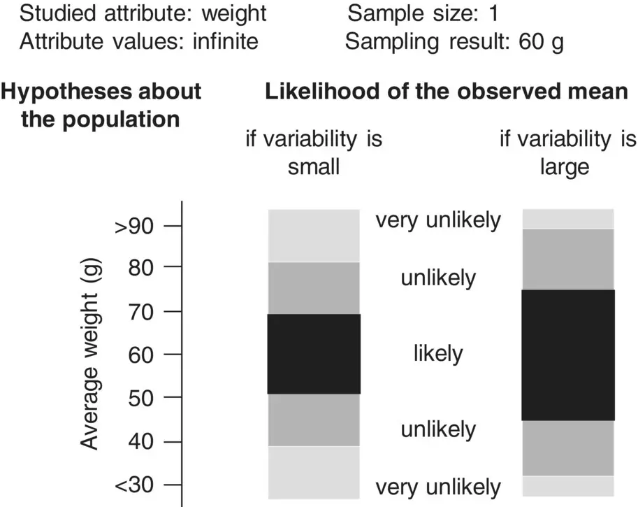
Figure 1.10 Inference with interval attributes II.

We have eliminated a lot of subjectivity by putting the notion of sample representativeness within a convenient framework. Now we must try to eliminate the remaining subjectivity in two other statements. First, we need to find a way to determine, objectively and reliably, the limits for population proportions and averages that are consistent with the samples. Second, we need to be more specific when we say that we are confident about those limits. Terms like confident, very confident, or quite confident lack objectivity, so it would be very useful if we could express quantitatively our degree of confidence in the estimates. In order to do that, as we have seen, we need a measure of the variation of the values of an attribute.

As with the central tendency measures, there are a number of available measures of dispersion, each one having some useful properties and some shortcomings. One possible way of expressing the degree of heterogeneity of the values of an attribute could be to write down the limits, that is, the minimum and maximum values ( Figure 1.11). The limits are actually measures of location. These measures indicate the values on defined positions in an ordered set of values. One good thing about this approach is that it is easy to interpret. If the two values are similar then the dispersion of the values is small, otherwise it is large. There are some problems with the limits as measures of variation, though. First, we will have to deal with two quantities, which is not practical. Second, the limits are rather unstable, in the sense that if one adds a dozen observations to a study, most likely it will be necessary to redefine the limits. This is because, as one adds more observations, the more extreme values of an attribute will have a greater chance of appearing.

The first problem can be solved by using the difference between the maximum and minimum values, a quantity commonly called the range, but this will not solve the problem of instability.

The second problem can be minimized if, instead of using the minimum and maximum to describe the dispersion of values, we use the other measures of location, the lower and upper quartiles. The lower quartile (also called the 25th percentile) is the value below which one‐quarter, or 25%, of all the values in the dataset lie. The upper quartile (or 75th percentile) is the value below which three‐quarters, or 75%, of all the values in the dataset lie (note, incidentally, that the median is the same as the 50th percentile). The advantage of the quartiles over the limits is that they are more stable because the addition of one or two extreme values to the dataset will probably not change the quartiles.

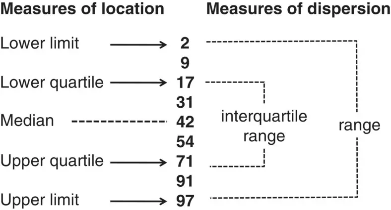
Figure 1.11 Measures of dispersion derived from measures of location.