A. Gouveia Oliveira - Biostatistics Decoded

These results are presented in the graph in Figure 1.32, which displays all possible proportions of females in samples of four and their relative frequency. Since, as we saw before, the proportion of females in a sample corresponds to the mean of that attribute, the graph is nothing more than the probability distribution of the sample proportions, the binomial distribution. All random binary attributes, like the proportion of patients with asthma in a sample, or the proportion of responses to a treatment, follow the binomial distribution.

Therefore, with interval attributes we know the probability distribution of sample means only when the sample sizes are large or the attribute has a normal distribution. By contrast, with binary attributes we always know which the probability distribution of sample proportions is: it is the binomial distribution.

The calculation of the frequency of all possible results by the method outlined above can be very tedious for larger sample sizes, because there are so many possible results. It is also complicated for attributes whose values, unlike the above example, do not have equal probability. Fortunately, there is a formula for the binomial distributionthat allows us to calculate the frequencies for any sample size and for any probability of the attribute values. The formula is:

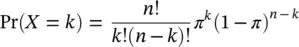
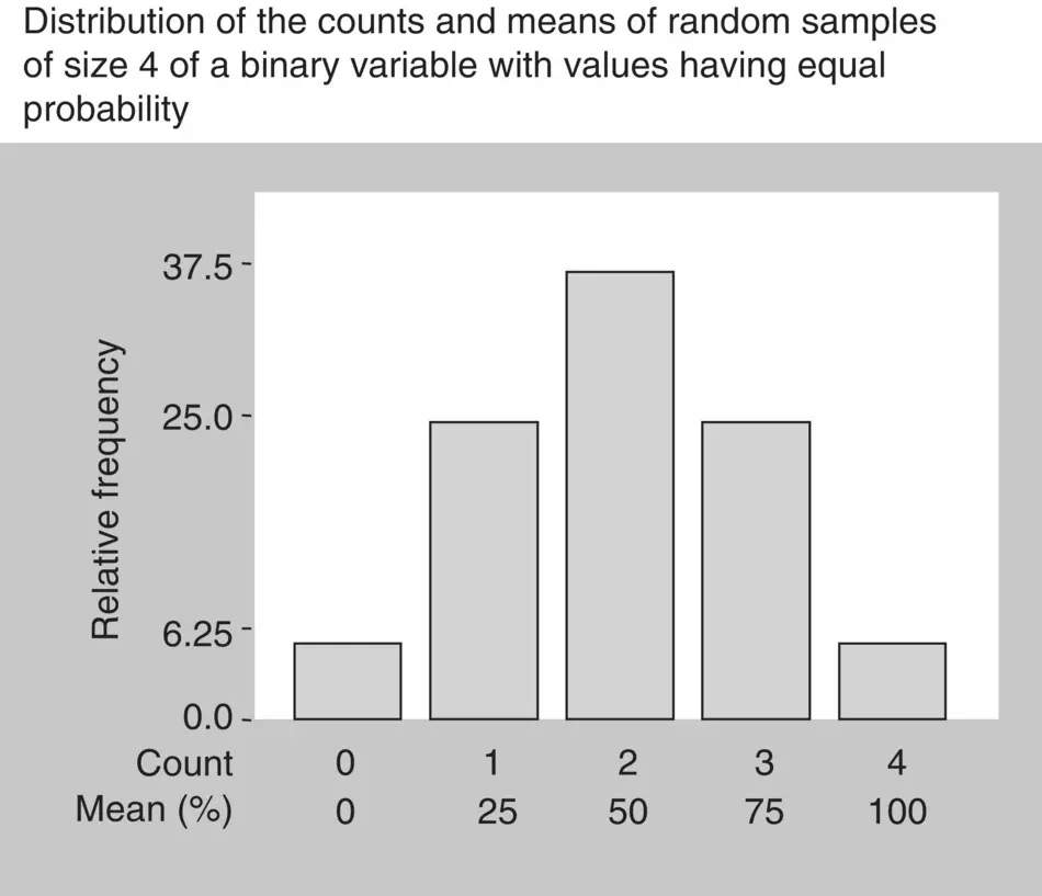
Figure 1.32 Probability distribution of a proportion: the binomial distribution.

We can use the formula to make the above calculations. For example, to calculate the probability of having k = 3 women in a sample of n = 4 observations, assuming that the proportion of women in the population is π = 0.5:

as before.

Since the means of binary attributes in random samples follow a probability distribution, we can calculate the mean and the variance of sample proportions in the same way as we did with interval‐scaled attributes. If we view a sample proportion as the sum of single observations from binary variables with identical distribution, then the properties of means allow us to conclude that the mean of the distribution of sample proportions is equal to the population proportion of the attribute.

By the same reasoning, we conclude that the variance of sample proportionsmust be the population variance of a binary attribute (the product of the probability of each value), divided by the sample size. If we call π the probability of an attribute having the value 1 (or, if we prefer, the proportion of the population having the attribute) and n the sample size, the variance of sample proportions is, therefore

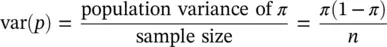
The standard deviation, which we call the standard error of sample proportions, is the square root of var( p ).

To sum up, let us review what can be said about the distribution of means of random samples of binary variables:

The distribution of the sample proportions is always known, and is called the binomial distribution.

The mean of the distribution of sample proportions is equal to the population proportion of the attribute.

The standard error of sample proportions is equal to the square root of the product of the probability of each value divided by the sample size.

If we view a sample proportion as the sum of single observations from binary variables with identical distribution, then the central limit theorem applies. Therefore, as the sample size increases, the distribution of sample proportions will approach the normal distribution and, if the sample size is large enough, the two distributions will almost coincide. This is called convergence of probability distributions. The convergence of the binomial distribution to the normal distribution as the sample size increases can be confirmed visually in Figure 1.33.

What is the minimum sample size above which the normal approximation to the binomial distribution is adequate is a matter of debate. When n increases, the convergence is faster for proportions around 0.5 and slower for proportions near 0.1 or 0.9, so the proportion must be taken into account. One commonly used rule of thumb is that a good approximation can be assumed when there are at least five observations with, and at least five without, the attribute. This means that if the proportion is 50%, then a sample of 10 will be enough, but if the proportion is 1% or 99%, then the sample must be about 500 observations. Other rules say that there must be at least nine observations with each value of the attribute.

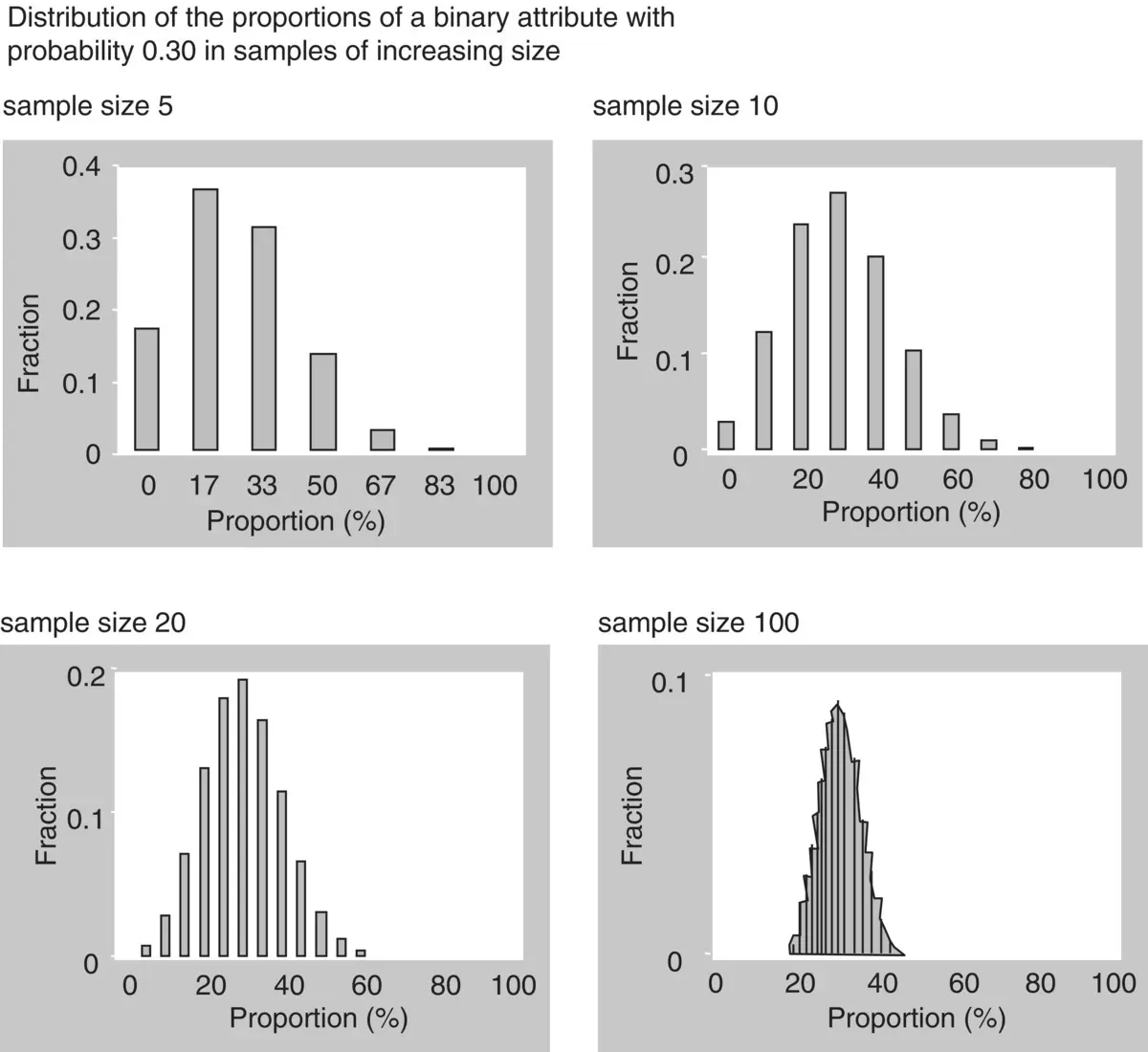
Figure 1.33 The convergence of the binomial to the normal distribution.

Текст предоставлен ООО «ЛитРес».

Прочитайте эту книгу целиком, на ЛитРес.

Безопасно оплатить книгу можно банковской картой Visa, MasterCard, Maestro, со счета мобильного телефона, с платежного терминала, в салоне МТС или Связной, через PayPal, WebMoney, Яндекс.Деньги, QIWI Кошелек, бонусными картами или другим удобным Вам способом.