A. Gouveia Oliveira - Biostatistics Decoded

From all of the above, we can conclude the following about sampling distributions:

Sample means have a normal distribution, regardless of the distribution of the attribute, but on the condition that they are large.

Small samples have a normal distribution only if the attribute has a normal distribution.

The mean of the sample means is the same as the population mean, regardless of the distribution of the variable or the sample size.

The standard deviation of the sample means, or standard error, is equal to the population standard deviation divided by the square root of the sample size, regardless of the distribution of the variable or the sample size.

Both the standard deviation and the standard error are measures of dispersion: the first measures the dispersion of the values of an attribute and the second measures the dispersion of the sample means of an attribute.

The above results are valid only if the observations in the sample are mutually independent.

Let us continue to view, as in Section 1.17, the sample mean as a random variable that results from the sum of identically distributed independent variables. The mean and variance of each of these identical variables are, of course, the same as the population mean and variance, respectively μ and σ 2.

When we compute sample means, we sum all observations and divide the result by the sample size. This is exactly the same as if, before we summed all the observations, we divided each one by the sample size. If we represent the sample mean by m , each observation by x , and the sample size by n , what was just said can be represented by

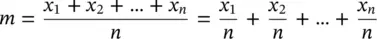
This is the same as if every one of the identical variables was divided by a constant amount equal to the sample size. From the properties of means, we know that if we divide a variable by a constant, its mean will be divided by the same constant. Therefore, the mean of each x i/ n is equal to the population mean divided by n , that is, μ / n .

Now, from the properties of means we know that if we add independent variables, the mean of the resulting variable will be the sum of the means of the independent variables. Sample means result from adding together n variables, each one having a mean equal to μ / n . Therefore, the mean of the resulting variable will be n × μ / n = μ , the population mean. The conclusion, therefore, is that the distribution of sample means m has a mean equal to the population mean μ .

A similar reasoning may be used to find the value of the variance of sample means. We saw above that, to obtain a sample mean, we divide every single identical variable x by a constant, the sample size n . Therefore, according to the properties of variances, the variance of each identical variable x i/ n will be equal to the population variance σ 2divided by the square of the sample size, that is, σ 2/ n 2. Sample means result from adding together all the x . Consequently, the variance of the sample mean is equal to the sum of the variances of all the observations, that is, equal to n times the population variance divided by the square of the sample size:

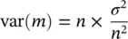
This is equivalent to σ 2/ n , that is, the variance of the sample means is equal to the population variance divided by the sample size. Therefore, the standard deviation of the sample means (the standard error of the mean) equals the population standard deviation divided by the square root of the sample size.

One must not forget that these properties of means and variances only apply in the case of independent variables. Therefore, the results presented above will also only be valid if the sample consists of mutually independent observations. On the other hand, these results have nothing to do with the central limit theorem and, therefore, there are no restrictions related to the normality of the distribution or to the sample size. Actually, whatever the distribution of the attribute and the sample size might be, the mean of the sample means will always be the same as the population mean, and the standard error will always be the same as the population standard deviation divided by the square root of the sample size, provided that the observations are independent. The problem is that, in the case of small samples from an attribute with unknown distribution, we cannot assume that the sample means will have a normal distribution. Therefore, knowledge of the mean and of the standard error will not be sufficient to completely characterize the distribution of sample means.

So far we have discussed the distribution of sample means of interval variables. What happens with sample means of binary variables when we take samples of a given size n from the same population?

We will repeat the experiment that was done for interval variables but now we will generate a random binary variable with probability 0.30 and take many samples of size 60. Of course, we will observe variation of the sample proportions as we did with sample means, as shown in Figure 1.31. As before, let us plot the sample proportions to see if there is a pattern for the distribution of their values.

The resulting graph is different from the one we obtained with sample means of interval variables. It clearly is not symmetrical, but above all the probability distribution is not continuous, it is discrete. Although resembling the normal distribution, this one is a different theoretical probability distribution, called the binomial distribution.

We shall now see how to create a binomial distribution. Imagine samples of four random observations on a binary attribute, such as sex, for example, which we know that the distribution in a population is equally divided between males and females. Each sample may have from 0 to 4 females, so the proportion of females in the samples is 0, 25, 50, 75, or 100%.

It is a simple matter to calculate the frequency with which each of these results will appear. We write down all possible combinations of males and females that can be obtained in samples of four, and count in how many cases there are 0, 1, 2, 3, and 4 females. In this example, there are 16 possible outcomes. There is only one way of having 0 females, so the theoretical relative frequency of this outcome is once out of 16 outcomes, or 6.25%. There are four possible ways out of 16 of having 25% of females, which is when the first, or the second, or the third, or the fourth sampled individual is a female. Hence, the relative frequency of this outcome, at least theoretically, is 25%. There are six possible ways of having 50% of females, so the relative frequency of this outcome is 37.5%. There are four possible ways of having 75% of females, so the frequency of this result is 25%. Finally, there is only one possible way of having 100% of females, and the relative frequency of this result is 6.25%.

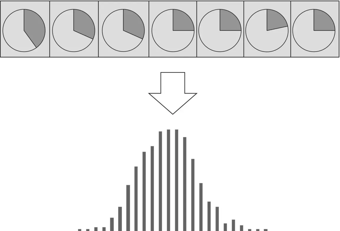
Figure 1.31 Illustration of the phenomenon of sampling variation. Above, pie charts show the observed proportions in random samples of size n of a binary variable. The graph below shows the distribution of sample proportions of a large number of random samples.