A. Gouveia Oliveira - Biostatistics Decoded

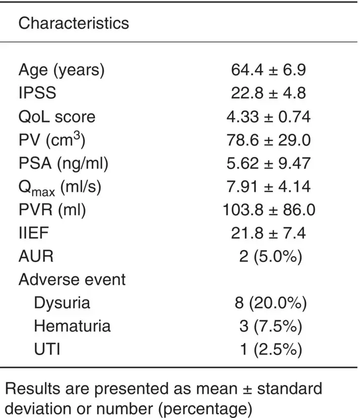
Figure 1.21 Table with summary statistics describing the information collected from a sample.

Why data analysis does not stop after descriptive statistics are obtained from the data? After all, we have obtained population estimates of means and proportions, which is the information we were looking for. Probably that is the thinking of many people who believe that they have to present a statistical analysis otherwise they will not get their paper published.

Actually, sample means and proportions are even called point estimatesof a population mean or proportion, because they are unbiased estimators of those quantities. However, that does not mean that the sample mean or sample proportion has a value close to the population mean or the population proportion. We can verify that with a simple experiment.

Let us consider for now only sample means from interval variables. With the random number generator of the computer we can create an interval variable and obtain a number of random samples of identical size n of that variable. Figure 1.22shows some of the results of that experiment, displaying the plots of consecutive samples from an interval variable, with a horizontal line representing the sample means. It is quite clear that the sample means have a different value every time a sample is taken from a population. This phenomenon is called sampling variation.

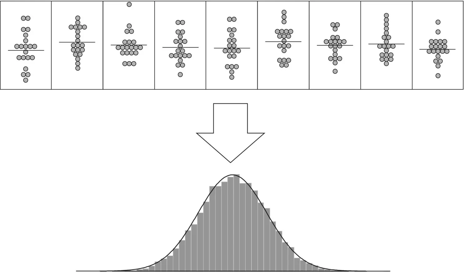
Figure 1.22 Illustration of the phenomenon of sampling variation. Above are shown plots of the values in random samples of size n of an interval variable. Horizontal lines represent the sample means. Below is shown a histogram of the distribution of sample means of a large number of random samples. Superimposed is the theoretical curve that would be obtained if an infinite number of sample means were obtained.

Now let us continue taking random samples of size n from that variable. The means will keep coming up with a different value every time. So we plot the means in a histogram to see if there is some discernible pattern in the frequency distribution of sample means. What we will eventually find is the histogram shown in Figure 1.22. If we could take an infinite number of samples and plotted the sample means, we would end up with a graph with the shape of the curve in the same figure.

What we learn from that experiment is that the means of interval attributes of independent samples of a given size n , obtained from the same population, are subjected to random variation. Therefore, sample means are random variables, that is, they are variables because they can take many different values, and they are random because the values they take are determined by chance.

We also learn, by looking at the graph in Figure 1.22, that sample means can have very different values and we can never assume that the population mean has value close to the value of the sample mean. Those are the reasons why we cannot assume that the value of the population mean is the same as the sample mean. So an important conclusion is that one must never, ever draw conclusions about a population based on the value of sample means. Sample means only describe the sample, never the population.

There is something else in the results of this experiment that draws attention: the curve representing the distribution of sample means has a shape like a hat, or a bell, where the frequency of the individual values is highest near the middle and declines smoothly from there and at the same rate on either side. The interesting thing is that we have seen a curve like this before. Of course, we could never obtain a curve like this because there is no way we can take an infinite number of samples. Therefore, that curve is theoretical and is a mathematical function that describes the probability of obtaining the values that a random variable can take and, thus, is called a probability distribution.

Figure 1.23presents several histograms showing the frequency distribution of several commonly assessed clinical laboratory variables measured in interval scales, obtained from a sample of over 400 patients with hypertension. Notice not only that all distributions are approximately symmetrical about the mean, but also that the very shape of the histograms is strikingly similar.

Actually, if we went around taking some kind of interval‐based measurements (e.g. length, weight, concentration) from samples of any type of biological materials and plotted them in a histogram, we would find this shape almost everywhere. This pattern is so repetitive that it has been compared to familiar shapes, like bells or Napoleon hats.

In other circumstances, outside the world of mathematics, people would say that we have here some kind of natural phenomenon. It seems as if some law, of physics or whatever, dictates the rules that variation must follow. This would imply that the variation we observe in everyday life is not chaotic in nature, but actually ruled by some universal law. If this were true, and if we knew what that law says, perhaps we could understand why, and especially how, variation appears.

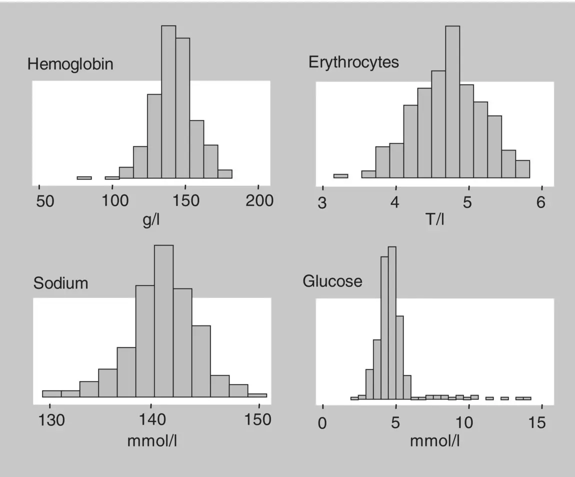
Figure 1.23 Frequency distributions of some biological variables.

So, what would be the nature of that law and is it known already? Yes it is, and it is actually very easy to understand how it works. Let us conduct a little experiment to see if we can create something whose values have a bell‐shaped distribution.

Consider some attribute that may take only two values, say 1 and 2, and those values occur with equal frequency. Technically speaking, we say a random variable taking values 1 and 2 with equal probability; this is the probability distribution for that variable (see Figure 1.24, upper part). Consider also, say, four variables that behave exactly like this one, that is, with the same probability distribution. Now let us create a fifth variable that is the sum of all four variables. Can we predict what will be the probability distribution of this variable?

We can, and the result is also presented in Figure 1.24. We simply write down all the possible combinations of values of the four equal variables and see in each case what the value of the fifth variable is. If all four variables have value 1, then the fifth variable will have value 4. If three variables have value 1 and one has value 2, then the fifth variable will have value 5. This may occur in four different ways – either the first variable had the value 2, or the second, or the third, or the fourth. If two variables have the value 1 and two have the value 2, then the sum will be 6, and this may occur in six different ways. If one variable has value 1 and three have value 2, then the result will be 7 and this may occur in four different ways. Finally, if all four variables have value 2, the result will be 8 and this can occur in only one way.

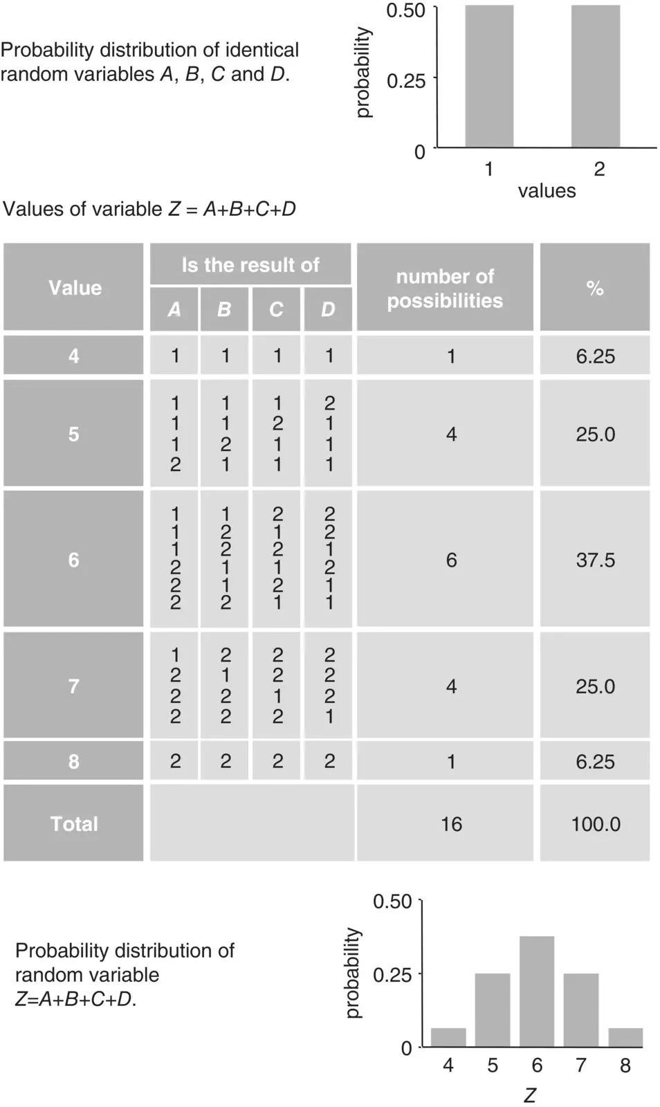
Figure 1.24 The origin of the normal distribution.