A. Gouveia Oliveira - Biostatistics Decoded

So, of the 16 different possible ways or combinations, in one the value of the fifth variable is 4, in four it is 5, in six it is 6, in four it is 7, and in one it is 8. If we now graph the relative frequency of each of these results, we obtain the graph shown in the lower part of Figure 1.24. This is the graph of the probability distribution of the fifth variable. Do you recognize the bell shape?

If we repeat the experiment with not two, but a much larger number of variables, the variable that results from adding all those variables will have not just five different values, but many more. Consequently, the graph will be smoother and more bell‐shaped. The same will happen if we add variables taking more than two values.

If we have a very large number of variables, then the variable resulting from adding those variables will take an infinite number of values and the graph of its probability distribution will be a perfectly smooth curve. This curve is called the normal curve. It is also called the Gaussian curveafter the German mathematician Karl Gauss who described it.

What was presented in the previous section is known as the central limit theorem. This theorem simply states that the sum of a large number of independent variables with identical distribution has a normal distribution. The central limit theorem plays a major role in statistical theory, and the following experiment illustrates how the theorem operates.

With a computer, we generated random numbers between 0 and 1, obtaining observations from two continuous variables with the same distribution. The variables had a uniform probability distribution, which is a probability distribution where all values occur with exactly the same probability.

Then, we created a new variable by adding the values of those two variables and plotted a histogram of the frequency distribution of the new variable. The procedure was repeated with three, four, and five identical uniform variables. The frequency distributions of the resulting variables are presented in Figure 1.25.

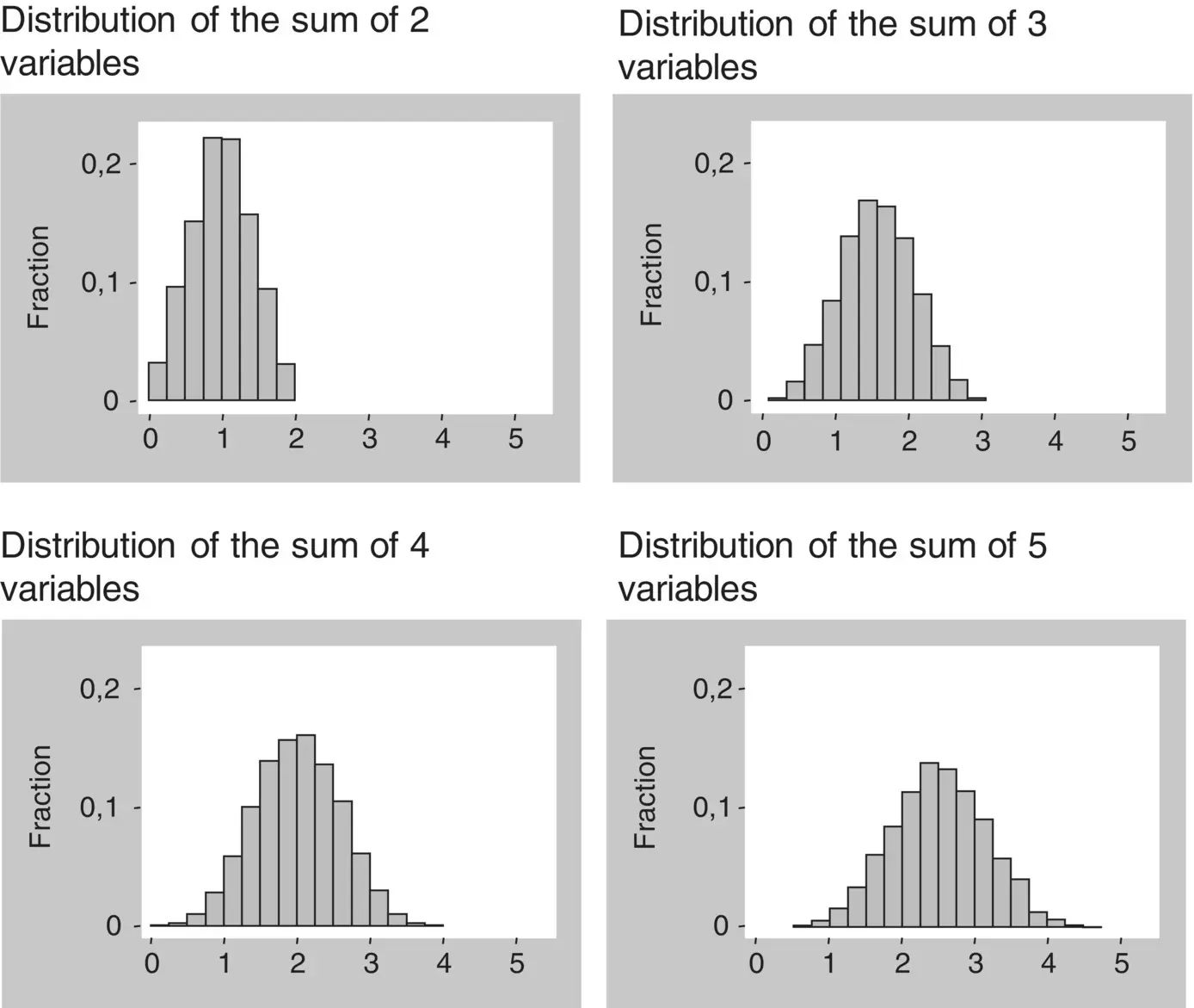
Figure 1.25 Frequency distribution of sums of identical variables with uniform distribution.

Notice that the more variables we add together, the more the shape of the frequency distribution approaches the normal curve. The fit is already fair for the sum of four variables. This result is a consequence of the central limit theorem.

The normal distribution has many interesting properties, but we will present just a few of them. They are very simple to understand and, occasionally, we will have to call on them further on in this book.

First property . The normal curve is a function solely of the mean and the variance. In other words, given only a mean and a variance of a normal distribution, we can find all the values of the distribution and plot its curve using the equation of the normal curve (technically, that equation is called the probability density function). This means that in normally distributed attributes we can completely describe their distribution by using only the mean and the variance (or equivalently the standard deviation). This is the reason why the mean and the variance are called the parametersof the normal distribution, and what makes these two summary measures so important. It also means that if two normally distributed variables have the same variance, then the shape of their distribution will be the same; if they have the same mean, their position on the horizontal axis will be the same.

Second property . The sum or difference of normally distributed independent variables will result in a new variable with a normal distribution. According to the properties of means and variances, the mean of the new variable will be, respectively, the sum or difference of the means of the two variables, and its variance will be the sum of the variances of the two variables ( Figure 1.26).

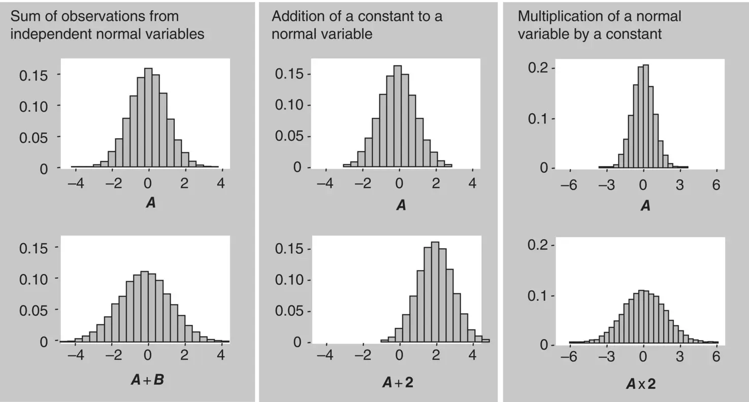
Figure 1.26 Properties of the normal distribution.

Third property . The sum, or difference, of a constant to a normally distributed variable will result in a new variable with a normal distribution. According to the properties of means and variances, the constant will be added to or subtracted from its mean, and its variance will not change ( Figure 1.26).

Fourth property . The multiplication, or division, of the values of a normally distributed variable by a constant will result in a new variable with a normal distribution. Because of the properties of means and variances, its mean will be multiplied, or divided, by that constant and its variance will be multiplied, or divided, by the square of that constant ( Figure 1.26).

Fifth property . In all normally distributed variables, irrespective of their means and variances, we can say that about two‐thirds of the observations have a value lying in the interval defined by the mean minus one standard deviation to the mean plus one standard deviation ( Figure 1.27). Similarly, we can say that approximately 95% of the observations have a value lying in the interval defined by the mean minus two standard deviations to the mean plus two standard deviations. The relative frequency of the observations with values between the mean minus three standard deviations and the mean plus three standard deviations is about 99%, and so on. Therefore, one very important property of the normal distribution is that there is a fixed relationship between the standard deviation and the proportion of values within an interval on either side of the mean defined by a number of standard deviations. This means that if we know that an attribute, for example, height, has normal distribution with a population mean of 170 cm and standard deviation of 20 cm, then we also know that the height of about 66% of the population is 150–190 cm, and the height of 95% of the population is 130–210 cm.

Recall what was said earlier, when we first discussed the standard deviation: that its interpretation was easy but not evident at that time. Now we can see how to interpret this measure of dispersion. In normally distributed attributes, the standard deviation and the mean define intervals corresponding to a fixed proportion of the observations. This is why summary statistics are sometimes presented in the form of mean ± standard deviation (e.g. 170 ± 20).

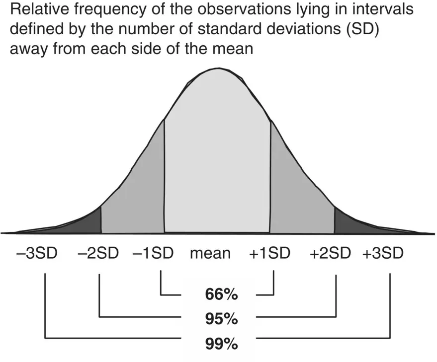
Figure 1.27 Relationship between the area under the normal curve and the standard deviation.

The reason for the pattern of variation of sample means observed in Section 1.13can easily be understood. We know that a mean is calculated by summing a number of observations on a variable and dividing the result by the number of observations. Normally, we look at the values of an attribute as observations from a single variable. However, we could also view each single value as an observation from a distinct variable, with all variables having an identical distribution. For example, suppose we have a sample of size 100. We can think that we have 100 independent observations from a single random variable, or we can think that we have single observations on 100 variables, all of them with identical distribution. This is illustrated in Figure 1.28. What do we have there, one observation on a single variable – the value of a throw of six dice – or one observation on each of six identically distributed variables – the value of the throw of one dice? Either way we look at it we are right.