Ashish Tewari - Foundations of Space Dynamics

(2.113)

whose substitution into the triple integrals in Eqs. ( 2.110) and ( 2.111) leads to the integration in the longitude, , being carried out independently of and as follows:

(2.114)

This implies that and

(2.115)

These simplifications allow the gravitational potential of an axisymmetric body to be expressed as follows:

(2.116)

where

(2.117)

A more useful expression for the gravitational potential can be obtained as follows in terms of the non‐dimensional distance, , where is the equatorial radius of the axisymmetric body:

(2.118)

where and

(2.119)

are called Jeffery's constants , and are unique for a body of a given mass distribution. Jeffery's constants represent the spherical harmonics of the mass distribution, and diminish in magnitude as the order, k , increases. The largest of these constants, , denotes a non‐dimensional difference between the moments of inertia about the polar axis, , and an axis in the equatorial plane ( or in Fig. 2.5), and is a measure of the ellipticity (or oblateness ) of the body. The higher order term, indicates the pear‐shaped or triangular harmonic, whereas and are the measures of square and pentagonal shaped harmonics, respectively. For a reasonably large body, it is seldom necessary to include more than the first four Jeffery's constants. For example, Earth's spherical harmonics are given by , and .

The acceleration due to gravity of an axisymmetric body is obtained by taking the gradient of the gravitational potential, Eq. (2.118), with respect to the position vector, , and can be resolved in the radial, , and the north polar, , directions (Fig. 2.5) as follows:

(2.120)

where the following identities have been employed:

The acceleration can be alternatively resolved in two mutually perpendicular directions, and (see Fig. 2.5). The unit vectors and denote the radial and southward directions, as shown in Fig. 2.5, while the unit vector signifies the direction of the increasing longitude; that is, the eastward direction. These unit vectors constitute a moving coordinate frame, , attached to the test mass as shown in Fig. 2.5. Such a frame is called a local‐horizon frame (see Chapter 5). The acceleration given by Eq. (2.120)is resolved in and by substituting 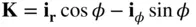, resulting in