Robert Bartoszynski - Probability and Statistical Inference
Здесь есть возможность читать онлайн «Robert Bartoszynski - Probability and Statistical Inference» — ознакомительный отрывок электронной книги совершенно бесплатно, а после прочтения отрывка купить полную версию. В некоторых случаях можно слушать аудио, скачать через торрент в формате fb2 и присутствует краткое содержание. Жанр: unrecognised, на английском языке. Описание произведения, (предисловие) а так же отзывы посетителей доступны на портале библиотеки ЛибКат.
- Название:Probability and Statistical Inference
- Автор:
- Жанр:
- Год:неизвестен
- ISBN:нет данных
- Рейтинг книги:4 / 5. Голосов: 1
-
Избранное:Добавить в избранное
- Отзывы:
-
Ваша оценка:
Probability and Statistical Inference: краткое содержание, описание и аннотация
Предлагаем к чтению аннотацию, описание, краткое содержание или предисловие (зависит от того, что написал сам автор книги «Probability and Statistical Inference»). Если вы не нашли необходимую информацию о книге — напишите в комментариях, мы постараемся отыскать её.
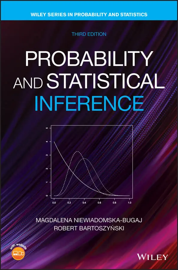
Probability and Statistical Inference, Third Edition
Probability and Statistical Inference
Probability and Statistical Inference — читать онлайн ознакомительный отрывок
Ниже представлен текст книги, разбитый по страницам. Система сохранения места последней прочитанной страницы, позволяет с удобством читать онлайн бесплатно книгу «Probability and Statistical Inference», без необходимости каждый раз заново искать на чём Вы остановились. Поставьте закладку, и сможете в любой момент перейти на страницу, на которой закончили чтение.
Интервал:
Закладка:
Problems
1 1.4.1 Let be a countable partition of ; that is, for all , and . Let . Find .
2 1.4.2 Assume that John will live forever. He plays a certain game each day. Let be the event that he wins the game on the th day. (i) Let be the event that John will win every game starting on January 1, 2035. Label the following statements as true or false: (a) . (b) . (c) . (d) . (ii) Assume now that John starts playing on a Monday. Match the following events through with events through : John loses infinitely many games. When John loses on a Thursday, he wins on the following Sunday. John never wins on three consecutive days. John wins every Wednesday. John wins on infinitely many Wednesdays. John wins on a Wednesday. John never wins on a weekend. John wins infinitely many games and loses infinitely many games. If John wins on some day, he never loses on the next day.
3 1.4.3 Let be distinct subsets of . (i) Find the maximum number of sets (including and ) of the smallest field containing . (ii) Find the maximum number of sets in this field if . (iii) Answer (ii) if . (iv) Answer (ii) if . (v) Answer (i)–(iv) for a ‐field.
4 1.4.4 For let . Consider a sequence of numbers satisfying for all , and let . (i) Find and . (ii) Find conditions, expressed in terms of , under which exists, and find this limit. (iii) Define and . Answer questions (i) and (ii) for sequence .
5 1.4.5 Let be the set of all integers. For , let be the number of elements in the intersection . Let be the class of all sets for which the limitexists. Show that is not a field. [Hint: Let and { all odd integers between and and all even integers between and for . Show that both and are in but .]
6 1.4.6 Let . Show that the class of all finite unions of intervals of the form and , with possibly infinite or (intervals of the form etc.) forms a field.
Notes
1 1Unless specifically stated, we will be assuming that all coins and/or dice tossed are fair (balanced).
2 2Asterisks denote more advanced material, as explained in the Preface to the Second Edition.
3 3In view of the fact proved earlier that all monotone sequences converge, this condition means that (a) if is an increasing sequence of sets in , then and (b) if is a decreasing sequence of sets in , then .
4 4For various relations among classes of sets defined through closure properties under operations, for example, see Chow and Teicher (1997) and Chung (2001).
Chapter 2 Probability
2.1 Introduction
The concept of probability has been an object of debate among philosophers, logicians, mathematicians, statisticians, physicists, and psychologists for the last couple of centuries, and this debate is not likely to be over in the foreseeable future. As advocated by Bertrand Russell in his essay on skepticism, when experts disagree, the layman would do best by refraining from forming a strong opinion. Accordingly, we will not enter into the discussion about the nature of probability; rather, we will start from the issues and principles that are commonly agreed upon.
Probability is a number associated with an event that is intended to represent its “likelihood,” “chance of occurring,” “degree of certainty,” and so on. Probabilities can be obtained in several ways, the most common being (1) the frequency (or objective ) interpretation, (2) the classical (sometimes called logical ) interpretation, and (3) the subjective or personal interpretation of probability.
2.2 Probability as a Frequency
According to the common interpretation, probability is the “long‐run” relative frequency of an event. The idea connecting probability and frequency is (and had been for a long time) very well grounded in everyday intuition. For instance, loaded dice were on several occasions found in the graves of ancient Romans. That indicates that they were aware of the possibility of modifying long‐run frequencies of outcomes, and perhaps making some profit in such a way.
Today, the intuition regarding relationship between probabilities and frequencies is even more firmly established. For instance, the phrases “there is 3% chance that an orange picked at random from this shipment will be rotten” and “the fraction of rotten oranges in this shipment is a 3%” appear almost synonymous. But on closer reflection, one realizes that the first phrase refers to the probability of an event “randomly selected orange will be rotten,” while the second phrase refers to the population of oranges.
The precise nature of the relation between probability and frequency is hard to formulate. But the usual explanation is as follows: Consider an experiment that can be repeated under identical conditions, potentially an infinite number of times. In each of these repetitions, some event, say  , may occur or not. Let
  be the number of occurrences of
  in the first
  repetitions. The frequency principle states that the ratio
  approximates the probability
  of event
  , with the accuracy of the approximation increasing as
  increases.
Let us observe that this principle serves as a basis for estimating probabilities of various events in the real world, especially those probabilities that might not be attainable by any other means (e.g., the probability of heads in tossing a biased coin).
We start this chapter by putting a formal framework (axiom system) on a probability regarded as a function on the class of all events . That is, we impose some general conditions on a set of individual probabilities. This axiom system, due to Kolmogorov (1933), will be followed by the derivation of some of its immediate consequences. The latter will allow us to compute probabilities of some composite events given the probabilities of some other (“simpler”) events.
2.3 Axioms of Probability
Let  be the sample space, namely the set of all outcomes of an experiment. Formally, probability, to be denoted by
  , is a function defined on the class of all events, 1 satisfying the following conditions (usually referred to as axioms ):
Axiom 1 (Nonnegativity):
Axiom 2 (Norming):

Axiom 3 (Countable Additivity):
Читать дальшеИнтервал:
Закладка:
Похожие книги на «Probability and Statistical Inference»
Представляем Вашему вниманию похожие книги на «Probability and Statistical Inference» списком для выбора. Мы отобрали схожую по названию и смыслу литературу в надежде предоставить читателям больше вариантов отыскать новые, интересные, ещё непрочитанные произведения.


Обсуждение, отзывы о книге «Probability and Statistical Inference» и просто собственные мнения читателей. Оставьте ваши комментарии, напишите, что Вы думаете о произведении, его смысле или главных героях. Укажите что конкретно понравилось, а что нет, и почему Вы так считаете.