Michael H. Veatch - Linear and Convex Optimization

5 Verification and validation. This step tries to determine if the model is an adequate representation of the decision problem. Verification involves checking for internal consistency in that the mathematical model agrees with its specification or assumptions. Validation seeks to build confidence that the model is sufficiently accurate. For optimization problems, accuracy may be gauged by whether the optimal solution produced by the model is reasonable or whether the objective function is accurate over a variety of feasible solutions. Validation methods that have been developed for statistical or simulation models might also be used.

6 Implementation. Once an optimal solution is obtained from the model, it may need to be modified. For example, fractional values may need to be converted to integers. The result may be one or more near‐optimal solutions that are presented to the decision‐maker. In other situations, the model may provide insights that help the decision‐maker with their decisions, or a system might be implemented so that the model is run repeatedly with new data to support future decisions.

These steps are not just done in this order. The verification and validation process, feedback obtained about the model, and changing situations often lead to multiple cycles of revising the model. When applications are presented in this book, we focus on Step 3, model formulation, and mostly on the translation process, not the simplifying assumptions. Whether a model is useful, however, depends on the other steps. It is important to ask “Where does the data come from?” as in Albright and Winston (2005). But it is also necessary to ask “Where does the model come from?,” that is, what are the model assumptions and why were they made?

Now we introduce more terminology for constrained optimization problems, as well as summarizing the terms introduced in the last section. These problems are called mathematical programs . The variables that we optimize over are the decision variables . They may be continuous variables , meaning that they can take on values in the real numbers, including fractions, or they may discrete variables that can only take on integer values. The function being optimized is the objective function . The domain over which the function is optimized is the set of points that satisfy the constraints, which can be equations or inequalities. We distinguish two kinds of constraints. Functional constraints can have any form, while variable bounds restrict the allowable values of one variable. Many problems have nonnegativity constraints as their variable bounds. In ( 1.1), the food constraint is listed with the functional constraints, making three functional constraints plus two nonnegativity constraints (variable bounds), but it is also a bound, so the problem can also be said to have two functional constraints and three bounds.

Let be the decision variables and satisfies the constraints be the solution set of the constraints. Departing somewhat from the usual meaning of a “solution” in mathematics, we make the following definitions

A solution to a mathematical program is any value of the variables.

A feasible solution is a solution that satisfies all constraints, i.e. .

The feasible region is the set of feasible solutions, i.e. .

The value of a solution is its objective function value.

An optimal solution is a feasible solution that has a value at least as large (if maximizing) as any other feasible solution.

To solve a mathematical program is to find an optimal solution and the optimal value , or determine that none exists. We can classify each mathematical program into one of three categories.

Existence of Optimal SolutionsWhen solving a mathematical program:

The problem has one or more optimal solutions (we include in this category having solutions whose value is arbitrarily close to optimal, but this distinction is rarely needed), or

The problem is an unbounded problem, meaning that, for a maximization, there is a feasible solution with value for every , or

The problem is infeasible: there are no feasible solutions, i.e. .

An unbounded problem, then, is one whose objective function is unbounded on (unbounded above for maximization and below for minimization). One can easily specify constraints for a decision problem that contradict each other and have no feasible solution, so infeasible problems are commonplace in applications. Any realistic problem could have bounds placed on the variables, leading to a bounded feasible region and a bounded problem. In practice, these bounds are often omitted, leaving the feasible region unbounded. A problem with an unbounded feasible region will still have an optimal solution for certain objective functions. Unbounded problems , on the other hand, indicate an error in the formulation. It should not be possible to make an infinite profit, for example.

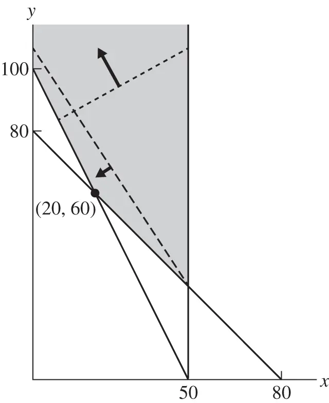
Figure 1.3Problem has optimal solution for dashed objective but is unbounded for dotted objective.

Example 1.1 (Unbounded region)Consider the linear program

(1.3)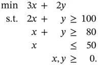

The feasible region is shown in Figure 1.3; the dashed line has an objective function value of 210. Sweeping this line down, the minimum value occurs at the corner point with an optimal value of 180. The feasible region is unbounded. Now suppose the objective function is changed to . The dotted line shows the contour line ; sweeping the line upward decreases the objective without bound, showing that the problem is unbounded.