Eleftheria Papadimitriou - Statistical Methods and Modeling of Seismogenesis

[1.20]

where Mmax is the upper limit of magnitude distribution (e.g. Cosentino et al . 1977).

The great popularity of the model [1.19]stems from two facts. First, it is a one-parameter model with a very simple form, and its parameter can be readily estimated, even from poorly populated samples. Second, the linear Gutenberg–Richter relation, at first glance, seems to fit almost all seismicity cases. This caused the Gutenberg–Richter relation to often be considered as a universal law, though there were works indicating breaks in scaling in the frequency-magnitude (early examples: Schwartz and Coppersmith 1984; Davison and Scholz 1985; Pacheco et al . 1992). The fit of the Gutenberg–Richter relation, and thus of the models [1.19]and [1.20]to actual earthquake samples, was rarely verified by rigorous statistical testing, and visible deviations from the model were interpreted as statistical scatter.

For obvious reasons, in seismic hazard problems, the attention is devoted to stronger magnitudes, whose exceedance probability, 1− FM ( M ), is low. This exceedance probability of magnitude enters the equations characterizing hazards in either the negative exponent (equations [1.16]and [1.17]), or in the denominator ( equation [1.18]). When a magnitude distribution model was inappropriate in the range of larger magnitudes, this would result in significant systematic errors of hazard parameters.

There are parametric alternatives to the exponential models [1.19]and [1.20](see, e.g., Lasocki 1993; Utsu 1999, and the references therein; Jackson and Kagan 1999; Kagan 1999; Pisarenko and Sornette 2003). The drawback in all of them is that their PDFs either decrease monotonically, or have at most one mode, that is, one local maximum at the catalog completeness level, MC . Such distributions cannot correctly model the modes at larger magnitudes and faster than linear drops of the logarithmic number of observations in the range of larger magnitudes, that is, the features observed and expected based on physical models of seismicity. The same drawback holds for the exponential distribution model.

Two approaches can be proposed for investigating how well the exponential models [1.19]and [1.20]fit data. Within the first approach, the null hypothesis is H0 ( the magnitude distribution is exponential ) against the alternative that it is not exponential. This hypothesis can be readily assessed by means of the Kolmogorov-Smirnov one-sample test, or with better precision by the Anderson- Darling test. These tests can also verify some of the mentioned alternative models. When we estimate model parameters from the data sample, and then this model is tested, the Kolmogorov-Smirnov test statistics should be modified. Both tests are very popular but will not be described here. Examples of when the above null hypothesis was disproved can be found in Urban et al . (2016) and Leptokaropoulos (2020). It is worth noting that both tests are suitable for continuous random variables, whose samples do not contain repeated values. Magnitude is a continuous random variable, but in seismic catalogs magnitudes have a limited number of digits, usually one digit after the decimal point. Therefore, magnitude data samples have many repetitions. To remedy the problem, Lasocki and Papadimitriou (2006) recommended randomizing the data before testing through the following equation:

[1.21]

where M is the magnitude value taken from catalog, δM is the length of the magnitude round off interval, u is the random value drawn from the uniform distribution in the [0,1] interval, F (•) is the CDF of an exponential model fitting the data, F -1(•) denotes its inverse function and M *is the randomized value of magnitude. This randomization procedure will return the original catalog magnitude when M *is rounded to δM , and the randomized values in every interval [ M -0.5 δM , M +0.5 δM ] repeat exponential distribution of the whole dataset. We can object that the best fitted exponential distribution is used first to randomize the data, and next, this fit is tested. Indeed, this randomization slightly amplifies the probability that H0 will not be rejected. However, other randomizations, e.g., the one assuming normal distribution in [ M− 0.5 δM , M +0.5 δM ], is logically incorrect and strongly acts against H0.

Within the second approach, two independent null hypotheses are checked: H01 ( the magnitude distribution is at most unimodal) and H02 ( the number of bumps in the magnitude density ≤ 1). A bump is an interval [ a , b ] such that the probability density is concave over [ a , b ] but not over any larger interval. PDFs with two modes and two bumps, respectively, are illustrated in Figure 1.3.

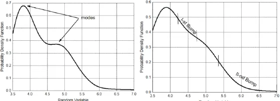
Figure 1.3. Left – PDF with two modes. Right – PDF with two bumps. Reprinted from Lasocki and Papadimitriou (2006, Figure 1)

This approach is suitable to test the applicability of the exponential model, as well as the above-mentioned alternatives, because all of these models have at most, one mode.

These two null hypotheses, H01 and H02, are studied using the smooth bootstrap test for multimodality presented by Silverman (1986) and Efron and Tibshirani (1993), with some adaptations to the magnitude distribution problem provided by Lasocki and Papadimitriou (2006). Given the magnitude data sample { M i}, i = 1,.., N , the procedure consists of the following steps:

– Step 1. Estimating the catalog (sample) completeness level, MC. We can do this either visually, selecting MC as the smallest magnitude of the linear part of the semi-logarithmic magnitude-frequency graph, or using more sophisticated methods presented, e.g., in Mignan and Woessner (2012), Leptokaropoulos et al. (2013) and the references therein.

– Step 2. Reducing the sample to its complete part {Mi|Mi ≥ Mc}, i = 1,.., n .

– Step 3. Estimating the exponential model of magnitude distribution [1.19]. The maximum likelihood estimator of β is (Aki 1965; Bender 1983):

[1.22]

where 〈 M 〉 stands for the mean value of the reduced (complete) sample, and the other symbols are the same as previously.

– Step 4. Randomizing {Mi}, i = 1,.., n according to equation [1.21], in which F(•) is CDF of the exponential distribution with parameter . The result is

The next steps begin from the kernel density estimate of magnitude, equation [1.3]. As it is shown in Figure 1.2, the number of modes and bumps of a kernel estimate depends on the bandwidth value, h . The greater h is, the fewer modes/bumps occur. Thus, there exists a critical value of bandwidth, hcrit , such that only has one mode for h ≥ hcrit and more than one mode for h < hcrit . Similarly for bumps. The critical bandwidths are denoted by for modes and bumps, respectively.