Eleftheria Papadimitriou - Statistical Methods and Modeling of Seismogenesis

The j -th jackknife sample, j ≤ n , is the n − 1 element sample { M 1, M 2,.., M j−1, M j+1, .., M n} that is the initial sample from which the j -th element has been removed. Hence, we can have, at most, n jackknife samples.

The first-order smoothed bootstrap samples are obtained in the same way as previously ( equation [1.25]). The k -th smoothed bootstrap sample, ℳ (k), is composed of:

[1.33]

where is the standard bootstrap sample obtained by n times uniform selection, with replacement from the original data { M i}, i = 1,.., n , and εi are the standard normal random numbers. We can have any number of the first-order bootstrap samples.

The second-order smoothed bootstrap samples are based on the first-order bootstrap sample, say ℳ (k), and the CDF kernel estimate from ℳ (k), say built on the bandwidth from [1.10], h (k), and weights from [1.7]. A j -th second-order smoothed bootstrap sample, ℳ (k,j), is composed of:

[1.34]

where is the standard bootstrap sample from ℳ (k).

The IBCa method can be presented in the following steps:

– Step 1. Generate n jackknife samples, estimate kernel CDF-s from the jackknife samples, and evaluate the accelerating constant:

[1.35]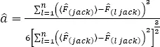

where stands for the arithmetic mean of

– Step 2. Generate B smoothed bootstrap samples of the first order, ℳ(k), k = 1,.., B, and estimate the kernel CDF-s from these samples,

– Step 3. From every first-order bootstrap sample generate BB smoothed bootstrap samples of the second order, ℳ(k,j), k = 1,.., B, j = 1,.., BB, and estimate the kernel CDF-s from these samples,

– Step 4. For every first-order bootstrap sample, ℳ(k), and its offspring second-order samples, ℳ(k,j), j = 1,.., BB, estimate the linked bias-correction parameter:

[1.36]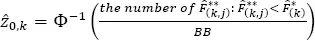

where Φ −1( • ) is the inverse function of the standard normal CDF. Calculate the bias-correction parameter as a mean value of the linked bias-correction parameters:

[1.37]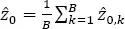

– Step 5. Calculate the orders of percentiles, α1 and α2:

[1.38]

where Φ( • ) is the standard normal CDF, and zα and z 1-αare percentiles of the standard normal distribution.

– Step 6. Sort in ascending order, The estimate of the confidence interval of length 1 − 2α for magnitude CDF is:

[1.39]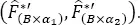

Orlecka-Sikora (2008) also provided a method to evaluate the optimal number of the first-order bootstrap samples, B . In general, B should be large, amounting tens of thousands for the initial sample of hundreds of elements. The reasonable number of the second-order samples is a few hundred for every first-order bootstrap sample. Hence, we have to generate tens of millions samples to get the confidence intervals [1.39]. Nevertheless, this is not a problem for high-performance computing (HPC).

When we assume that the seismic process is Poissonian and that the exact rate of earthquake occurrence, λ , is known, we readily obtain the confidence intervals for the exceedance probability and the mean return period. For the exceedance probability, R ( M , D ) ( equation [1.17]), it is:

[1.40]

and for the mean return period, T ( M ) ( equation [1.18]), it is:

[1.41]

Figure 1.6, taken from Orlecka-Sikora (2008), shows a practical example of the interval kernel estimation of CDF and the related hazard parameters. The studied seismic events were from Rudna deep copper mine in Poland and were parameterized in terms of seismic energy. Nevertheless, because the magnitude and the logarithm of energy have the same distribution, the specific features of the graphs in Figure 1.6would remain if magnitude was used.

Orlecka-Sikora and Lasocki (2017) presented a modified version of the interval estimation of R ( M , D ) ( equation [1.40]) and T ( M ) ( equation [1.41]), which also takes into account the uncertainty of earthquake occurrence rate, λ . It turned out that the uncertainty of λ only matters when λ D is small, less than 5. For greater λ D , the uncertainty of the CDF estimate dominates, and the role of the uncertainty of λ is negligible. In this connection, this modified version should mostly be used in hazard studies of low seismic activity regions.

Figure 1.6. Example of interval kernel estimation of CDF and related hazard parameters. The event size is parametrized by the logarithm of seismic energy. (a) CDF(logE) and its magnified part, (b) exceedance probability of logE=7.0 and (c) mean return period. Solid lines – the point kernel estimates (equations [1.32], [1.17] and [1.18]), dashed lines – the 95% confidence intervals from the Iterated BCa method. Reprinted from Orlecka-Sikora (2008, Figures 11, 14 and 15)