Eleftheria Papadimitriou - Statistical Methods and Modeling of Seismogenesis

[1.11]

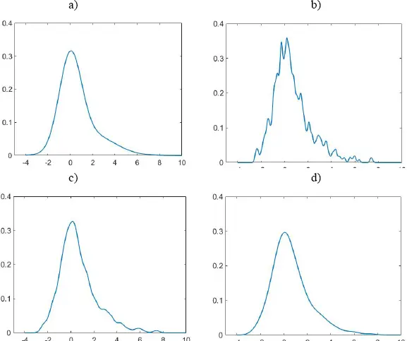
Figure 1.2. The dependence of density estimate on bandwidth, h. The actual distribution was the superposition of two normal distributions, 0.7 × NORM(0,1) + 0.3 × NORM(2,2). The exact PDF is presented in (a). The estimates were built from 500-element samples drawn from the actual distribution, using the normal kernel and constant bandwidths: (b) h = 0.1, (c) h = 0.25 and (d) h = 0.5. For a color version of this figure, see www.iste.co.uk/limnios/statistical.zip

When the interval [ x *, x *] is semi-finite, then the original sample is mirrored around and the sample or the sample is used to estimate The desired estimates of PDF and CDF are:

[1.12]

In connection with the above-mentioned problems with probabilistic functional models of earthquake parameters, the flexibility of kernel density estimation makes it a perfect tool for modeling the probabilistic distributions of such parameters. In particular, the kernel estimation method responds well to the needs of the PSHA.

The mathematical model in PSHA can be formulated, e.g., as the following expression for the probability that the ground motion amplitude parameter, amp , at the point ( x0 , y0 ), during D time units will exceed the value a ( x0 , y0 ):

Pr[ amp ( x 0, y 0) ≥ a ( x 0, y 0), D ] =

[1.13]

where r ( x0 , y0 ) is the epicentral distance of an earthquake to the receiving point ( x0 , y0 ), M is the earthquake magnitude, N ( D ) is the number of earthquakes in D , Pr[ a m p ( x 0, y 0) ≥ a ( x 0, y 0)| M , r ] is the probability that amp will exceed a due to the earthquake of magnitude, M , being distanced from the receiving point of r , fr is the PDF of epicentral distance, f ( M | N ( D ) ≠ 0) is the probability density of earthquake magnitude, M , conditional upon earthquake occurrence in D and ℳ is its domain. fr is straightforwardly linked to the two-dimensional probability distribution of earthquake epicenters, fxy ( x , y ). fxy ( x , y ) and f ( M | N ( D ) ≠ 0) represent the properties of seismic source (source effect), and Pr[ a m p ( x 0, y 0) ≥ a ( x 0, y 0)| M , r ] represents the properties of the vibration transmission from the source to the receiving point (path and site effects).

The conditional probability of source magnitude, f ( M | N ( D ) ≠ 0), can be evaluated from the probability mass function (PMF) of the number of earthquakes in D time units, Pr[ N ( D )= n ], and the unconditional PDF, fM , and the CDF, FM , of magnitude:

[1.14]

Under the assumption that the seismic occurrence process is Poissonian, equation [1.14]becomes:

[1.15]

where λ is the rate of earthquake occurrence.

The seismic hazard is often only characterized by its source component, namely, by the probability that an earthquake of a magnitude greater than or equal to M occurs within D time units (the exceedance probability), R ( M , D ), or the expected average time between successive occurrences of earthquakes with magnitudes ≥ M (the mean return period), T ( M ). The exceedance probability reads:

[1.16]

If the seismic occurrence process is considered as Poissonian then:

[1.17]

and

[1.18]

The most often used model of magnitude distribution, f M( M ), F M( M ), results from the empirical Gutenberg–Richter relation, which predicts a linear dependence of the logarithm of the number of earthquakes with magnitudes greater than or equal to M on M . This yields a piecewise distribution of magnitude:

[1.19]

where β is the distribution parameter and MC is the magnitude value beginning from where all earthquakes have been statistically recorded and are in the earthquake catalog. MC is called the catalog completeness level. Earthquake magnitude represents the physical size of an earthquake; hence in an environment of finite dimensions, as seismogenic zones are, it cannot be unlimited. For this reason, among others, we often amend the model [1.19]with an endpoint. The upper-bounded model of magnitude PDF with a hard endpoint is: