Eleftheria Papadimitriou - Statistical Methods and Modeling of Seismogenesis

The kernel density estimation is a model-free estimation of probability functions of continuous random variables. The estimation is carried out solely from sample data.

There is no attempt here to comprehensively present the kernel density estimation method. A detailed description and the discussion of the method can be found in the textbooks by Silverman (1986), Wand and Jones (1995), Scott (2015) and in a multitude of high-level research papers. The method is also implemented in Matlab, R and Python, among others, and in many statistical packages. In this chapter, the author presents how this method has been applied to selected problems of seismology. This presentation begins with a short and simplified theoretical introduction. The kernel density estimation has been fast developing from both theoretical and practical sides; hence, the techniques presented here do not aspire to be optimal. There is plenty of space for future modifications and developments.

In the case of a univariate random variable X , and a constant kernel, the kernel estimator of the actual probability density function (PDF) of X , f X( x ), takes the form:

[1.1]

where { x i}, i = 1,.., n is the sample data, K (•) is the kernel function, which is a PDF symmetric about zero, and h is the bandwidth, whose value decides how much smoothing has been applied to the sample data.

In the presented seismological applications of the kernel density estimation, we use the normal kernel function:

[1.2]

For this kernel function, the kernel estimates of PDF and the cumulative distribution function (CDF, ) are, respectively:

[1.3]

[1.4]

where Ф(·) is the CDF of standard normal distribution.

As it will follow, the kernel method is used, among others, to estimate the magnitude distribution, whose distribution is exponential-like or light-tailed. Because of that, the tail values are sparse in a sample. Such sparsity can result in spurious irregularities in the estimate on tails, if a constant bandwidth is used. We can alleviate this problem by using an adaptive kernel with variable bandwidth. Because the estimates of magnitude distribution functions serve in the probabilistic seismic hazard analysis (PSHA), the quality of the estimate in the tail part is of utmost importance.

The adaptive kernel estimate of PDF used here takes the form:

[1.5]

and the estimate of CDF is:

[1.6]

where ωi are the local weights widening the bandwidth associated with the data points from the range where the data is sparse. The weights take the form:

[1.7]

where is the constant kernel PDF estimate in xi , equation [1.3], and g = The way in which the kernel estimate of PDF is composed and the difference between the estimation with a constant and a variable bandwidth are presented in Figure 1.1.

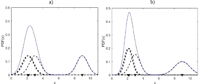
Figure 1.1. Buildup of the kernel estimate of PDF. Normal kernel functions (thick dashed lines) are associated with data points (triangles at abscissa). The PDF estimate (thin solid line) is the sum of the kernel functions. Whereas in the estimation with constant bandwidth, (a), all kernel functions are the same, in the estimation with variable bandwidth, (b), the kernels are wider in the regions of sparse data. For a color version of this figure, see www.iste.co.uk/limnios/statistical.zip

The final shape of the density estimate strongly depends on the value of h , which is demonstrated in the example in Figure 1.2. In the applications of the kernel estimators presented here, the criterion to select the bandwidth, h , is the minimizer of the mean integrated square error (MISE): where f is the actual (unknown) PDF, is its kernel estimate and E [•] denotes the expected value. Starting from MISE, Silverman (1986) derived the simplified score function of the form:

[1.8]

where K (•) is the kernel function, and Kijko et al . (2001) showed that for the normal kernel function, [1.2], the score function becomes:

[1.9]

and the bandwidth that minimizes M 1( h ) is the root of the equation:

[1.10]

When the random variable, for which the distribution functions are to be estimated, X , is defined over a finite or semi-finite interval, or its density is sharply zeroed outside a finite or semi-finite interval, the estimation of the distribution functions is modified according to Silverman (1986). Suppose that either X ∈ [ x *, x *], or the PDF, f X( x ), is not continuous in x *and x *, and f X( x ) = 0 for x < x *and x > x *. To get the kernel estimates of PDF and CDF, the original data sample, { x i}, i = 1,.., n , is mirrored symmetrically around x *and x *resulting in the sample {2 x *− x i, x i, 2 x *− x i}, i = 1,.. n . Based on this sample, a density is estimated and the desired estimates of PDF and CDF are: