Ian W. Hamley - Small-Angle Scattering
Здесь есть возможность читать онлайн «Ian W. Hamley - Small-Angle Scattering» — ознакомительный отрывок электронной книги совершенно бесплатно, а после прочтения отрывка купить полную версию. В некоторых случаях можно слушать аудио, скачать через торрент в формате fb2 и присутствует краткое содержание. Жанр: unrecognised, на английском языке. Описание произведения, (предисловие) а так же отзывы посетителей доступны на портале библиотеки ЛибКат.

- Название:Small-Angle Scattering
- Автор:
- Жанр:
- Год:неизвестен
- ISBN:нет данных
- Рейтинг книги:3 / 5. Голосов: 1
-
Избранное:Добавить в избранное
- Отзывы:
-
Ваша оценка:
Small-Angle Scattering: краткое содержание, описание и аннотация
Предлагаем к чтению аннотацию, описание, краткое содержание или предисловие (зависит от того, что написал сам автор книги «Small-Angle Scattering»). Если вы не нашли необходимую информацию о книге — напишите в комментариях, мы постараемся отыскать её.
A comprehensive and timely volume covering contemporary research, practical techniques, and theoretical approaches to SAXS and SANS Small-Angle Scattering: Theory, Instrumentation, Data, and Applications
Small-Angle Scattering: Theory, Instrumentation, Data, and Applications
Small-Angle Scattering — читать онлайн ознакомительный отрывок
Ниже представлен текст книги, разбитый по страницам. Система сохранения места последней прочитанной страницы, позволяет с удобством читать онлайн бесплатно книгу «Small-Angle Scattering», без необходимости каждый раз заново искать на чём Вы остановились. Поставьте закладку, и сможете в любой момент перейти на страницу, на которой закончили чтение.
Интервал:
Закладка:
( 1.95) 
In these equations J 0( qR ) and J 1( qR ) denote Bessel functions of integral order. The cross‐section radius is given by  [58] (see also the discussion in Section 1.4).
The pair distribution function of the cross‐section can be obtained from the cross‐section intensity via an inverse Hankel transform [7]
(1.96) 
For flat particles (discs of area A ) the intensity can be factored, via an equation analogous to Eq. (1.93)as [4, 6, 10]
( 1.97) 
where It ( q ) is the cross‐section scattering that depends on the thickness T , which is related to the cross‐section radius via  [58].
[58].
Expressions (1.93)and (1.97)indicate that as an alternative to the Guinier equation which provides Rg , the cylinder cross‐section radius can be obtained from a plot of ln[ qI ( q )] vs. q 2and for discs/planar structures Rc can be obtained a plot of ln[ q 2 I ( q )] vs. q 2[58, 59].
If the intensity is measured on an absolute scale it is possible to determine the mass per unit length for rod‐like particles or the mass per unit area for flat (lamellar) particles. The general expression for molar mass determination for an arbitrary particle from the differential scattering cross‐section d σ /dΩ in absolute units (cm −1) is discussed in Section 2.9. For rod‐like particles in a solution of concentration c (in g cm −3), the mass per unit length Mc (in g mol −1cm −1) can be obtained from the expression (containing a π/ q factor from Eq. (1.95))
(1.98) 
where NA is Avogadro's number, vp is the specific volume in cm 3g −1, Δρ is the contrast in cm −2and q is in cm −1.
For flat particles, the area per unit length Mt (in g mol −1cm −2) is obtained from the analogous equation (with q 2dependence cf. Eq. (1.93))
(1.99) 
The derivations of these equations can be found elsewhere [60].
1.7.4 Effect of Polydispersity
Particle polydispersity has a considerable influence on the shape of the form factor. It is included via integration over a particle size distribution D ( R′ ):
(1.100) 
Here the subscript 0 has been added to the form factor, in order to emphasize that this is the term for the monodisperse system.
The effect of polydispersity for the example of the form factor of a uniform sphere of radius R is illustrated in Figure 1.19. The polydispersity in this case is represented by a Gaussian function:
(1.101) 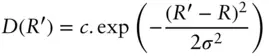
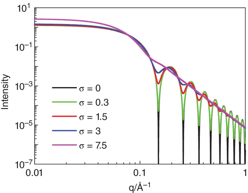
Figure 1.19 Influence of polydispersity on the form factor of a sphere with R = 30 Å in terms of a Gaussian standard deviation with width σ (in Å) indicated.
Here σ is the standard deviation, which is related to the full width at half maximum by  , and c is a normalization constant. Other forms of distribution can be used and may be motivated by known dispersity distributions (based on the system synthesis, for example), for example log‐normal functions, Schulz‐Zimm functions etc.
It is clear from the example of calculated form factors for a uniform sphere in Figure 1.19that increasing σ causes the form factor oscillations to get progressively washed out such that they are largely eliminated for σ = 7.5 Å (25% of the radius R ).
It can be difficult in some cases (in particular, when measurements extend over only a small q range and/or for highly polydisperse systems) to disentangle polydispersity from the effect of particle anisotropy, which can also smear out form factor minima. This is illustrated by the example of Figure 1.20which compares the calculated form factor for a sphere ( R = 30 Å, σ = 1.5) with that of a monodisperse ellipsoid with R 1= 29 Å and R 2= 34.8 Å. The form factors are quite similar at low q (and this example has not been optimized for maximal similarity). Especially with lower resolution SANS experiments (see Section 5.5.1for a discussion of the resolution function for SANS), the two profiles in Figure 1.20are not distinguishable at low q .
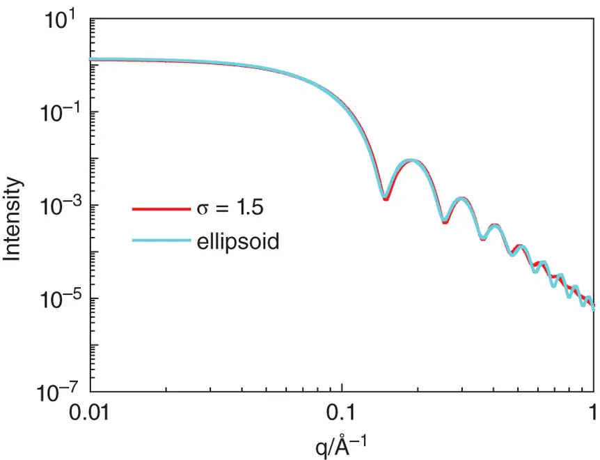
Figure 1.20 Comparison of form factor of a polydisperse sphere ( R = 30 Å, σ = 1.5) and a monodisperse ellipsoid with R 1= 29 Å and R 2= 34.8 Å.
1.8 FORM AND STRUCTURE FACTORS FOR POLYMERS
Polymers adopt coiled conformations. In the simplest picture, these are described as ideal Gaussian coils. Polymers in the melt or in solution (under theta conditions) adopt this conformation which is the most basic model of polymer conformation. The form factor for Gaussian coils can easily be calculated (as follows) to yield the Debye function. By analogy with Eq. (1.18), but integrating over a Gaussian distribution the intensity (form factor) is [61]
( 1.102) 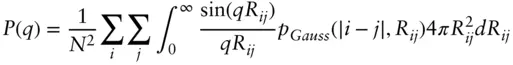
The Gaussian function for a random coil depends on the end‐to‐end distance between points i and j, R ijand | i – j |, which is the number of links between these points:
(1.103) 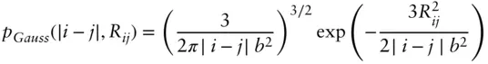
Интервал:
Закладка:
Похожие книги на «Small-Angle Scattering»
Представляем Вашему вниманию похожие книги на «Small-Angle Scattering» списком для выбора. Мы отобрали схожую по названию и смыслу литературу в надежде предоставить читателям больше вариантов отыскать новые, интересные, ещё непрочитанные произведения.


Обсуждение, отзывы о книге «Small-Angle Scattering» и просто собственные мнения читателей. Оставьте ваши комментарии, напишите, что Вы думаете о произведении, его смысле или главных героях. Укажите что конкретно понравилось, а что нет, и почему Вы так считаете.