Ian W. Hamley - Small-Angle Scattering
Здесь есть возможность читать онлайн «Ian W. Hamley - Small-Angle Scattering» — ознакомительный отрывок электронной книги совершенно бесплатно, а после прочтения отрывка купить полную версию. В некоторых случаях можно слушать аудио, скачать через торрент в формате fb2 и присутствует краткое содержание. Жанр: unrecognised, на английском языке. Описание произведения, (предисловие) а так же отзывы посетителей доступны на портале библиотеки ЛибКат.

- Название:Small-Angle Scattering
- Автор:
- Жанр:
- Год:неизвестен
- ISBN:нет данных
- Рейтинг книги:3 / 5. Голосов: 1
-
Избранное:Добавить в избранное
- Отзывы:
-
Ваша оценка:
Small-Angle Scattering: краткое содержание, описание и аннотация
Предлагаем к чтению аннотацию, описание, краткое содержание или предисловие (зависит от того, что написал сам автор книги «Small-Angle Scattering»). Если вы не нашли необходимую информацию о книге — напишите в комментариях, мы постараемся отыскать её.
A comprehensive and timely volume covering contemporary research, practical techniques, and theoretical approaches to SAXS and SANS Small-Angle Scattering: Theory, Instrumentation, Data, and Applications
Small-Angle Scattering: Theory, Instrumentation, Data, and Applications
Small-Angle Scattering — читать онлайн ознакомительный отрывок
Ниже представлен текст книги, разбитый по страницам. Система сохранения места последней прочитанной страницы, позволяет с удобством читать онлайн бесплатно книгу «Small-Angle Scattering», без необходимости каждый раз заново искать на чём Вы остановились. Поставьте закладку, и сможете в любой момент перейти на страницу, на которой закончили чтение.
Интервал:
Закладка:
The Fourier transform of the OZ equation is written as
( 1.75) 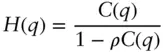
Where H ( q ) is the Fourier transform of h ( r ) and C ( q ) is the transform of c ( r ).
The structure factor is related to the pair correlation function g ( r ) via
( 1.76) 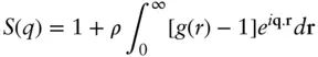
It may be noted that this equation differs from that given in Eq. (1.32)since the spherical average is not employed, and the normalization of g ( r ) differs.
Equation 1.76along with Eq. (1.75)lead to the OZ expression for the structure factor:
( 1.77) 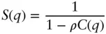
In the limit ρ → 0 the integral in Eq. (1.74)vanishes and the direct correlation function is [50]
( 1.78) 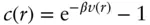
Here β = 1/ kB T . If βv ( r ) ≪ 1 Eq. (1.78)gives
(1.79) 
Which is known as the mean spherical approximation (MSA), used to evaluate the OZ equation.
The OZ equation can be solved using closure relationships for c ( r ) such as the hypernetted chain (HNC) approximation and the Percus‐Yevick (PY) approximation. The HNC equation is [50]
(1.80) 
or
(1.81) 
This simplifies to the MSA in the limit r → ∞ since h ( r ) → 0 in this limit, but generalized for any density.
The PY closure equation is given by
(1.82) 
This is obtained from an expansion of the HNC closure [50].
Exact solutions of these closure relationships are known, for instance using the PY approximation for hard spheres [50] or the Carnahan‐Starling approximation gives the expression in Eq. (1.38).
Further information on integral equation theories for liquids is available elsewhere [51].
1.7 FORM FACTORS
1.7.1 Examples of Form Factor Expressions
Analytical expressions are available for the form factor of particles of many geometries, as well as polymers discussed in Section 1.8. Some examples of more commonly used form factors are listed in Table 1.2. Extensive compilations of form factors are available [7, 17, 18, 21, 55].
Table 1.2 Expressions for common form factors.
| Form factor | Equation | Parameters |
|---|---|---|
| Homogeneous sphere |   |
Radius, R (  ), Scattering contrast, Δ ρ ), Scattering contrast, Δ ρ |
| Spherical shell | P ( q ) = [ Ks ( q , R 1, Δρ ) − Ks ( q , R 2, Δρ (1 − μ ))] 2 Ks ( q , R , Δ ρ ) as for a homogeneous sphere as above (other parameterizations are possible) | Outer radius R 1with shell scattering contrast Δ ρ Inner radius R 2with core scattering contrast Δ ρ (1− μ ) |
| Gaussian polymer chain –Debye function (see Section 1.8for derivation) | 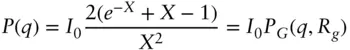 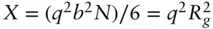 |
I 0, forward scattering intensity Rg , radius of gyration ( b , statistical segment length) |
| Sphere with attached Gaussian chains (used for block copolymer micelles) [52, 53] |  where where 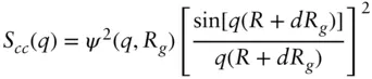 and and  with with 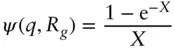 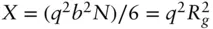 |
Nc , aggregation number R , core radius Rg , radius of gyration of attached chains d , displacement of chains (for non‐penetration into core, d ≈ 1) Δ ρs , scattering contrast of spherical core Δ ρc , scattering contrast of attached chains |
| Ellipsoid of revolution (spheroid) | 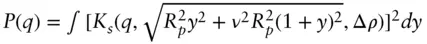 Ks ( q , R , Δ ρ ) as for a homogeneous sphere as above (other parameterizations are possible) Ks ( q , R , Δ ρ ) as for a homogeneous sphere as above (other parameterizations are possible) |
Radius in polar direction Rp Equatorial radius Re = νRp Scattering contrast, Δ ρ |
| Tri‐axial ellipsoid | P ( q ) = ∫ [ Ks ( q , R ( a , b , c , α , β , Δρ )] 2sin α d α d β R ( a , b , c , α , β ) =[( a 2sin 2 β + b 2cos 2 β )sin 2 α + c 2cos 2 α ] 1/2 Ks ( q , R , Δ ρ ) as for a homogeneous sphere as above (other parameterizations are possible) | Semi axis lengths a , b , c Scattering contrast, Δ ρ |
| Rectangular parallelepipedons (including cubes) |  Where Where 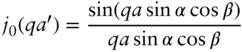 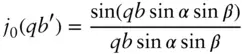 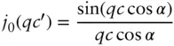 |
Edge lengths a , b , c Scattering contrast, Δ ρ |
| Circular cylinder | 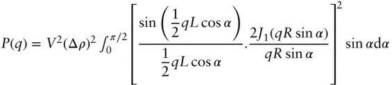 |
Radius, R . length, L . Scattering contrast, Δ ρ |
| Infinitely thin circular disc | 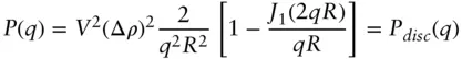 |
Radius, R Scattering contrast, Δ ρ |
| Lipid bilayer with Gaussian scattering density profile (within a disc) | P ( q ) = [ Pdisc ( q )/(Δ ρ ) 2] Pcs ( q ) where the cross‐section form factor Pcs ( q ) is 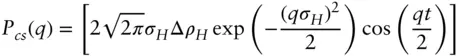 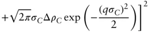 |
Cross‐section parameters illustrated in Figure 1.16 |
| Helices and helical tapes (Pringle–Schmidt form factor [54]) | 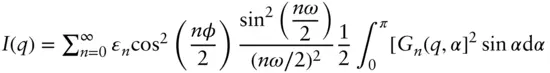 Here Here 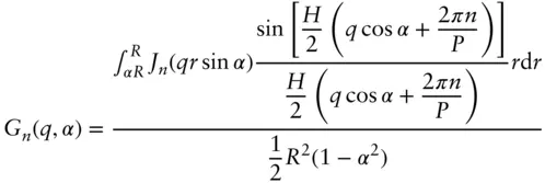 and ɛ 0= 1 and ɛn = 2 for n ≥ 1 and ɛ 0= 1 and ɛn = 2 for n ≥ 1 |
H helix length, P helix pitch, other parameters defined in Figure 1.16 |
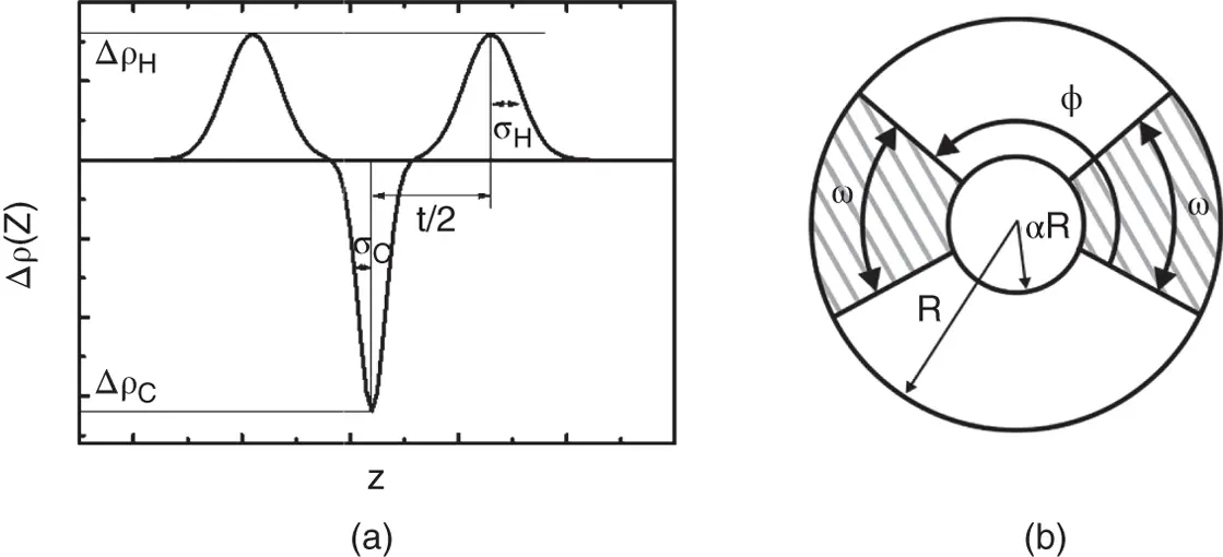
Figure 1.16 Parameters for complex form factors. (a) Gaussian bilayer, (b) Projection of a helical structure showing definitions of angles and radii in the corresponding Pringle–Schemidt form factor ( Table 1.2).
Читать дальшеИнтервал:
Закладка:
Похожие книги на «Small-Angle Scattering»
Представляем Вашему вниманию похожие книги на «Small-Angle Scattering» списком для выбора. Мы отобрали схожую по названию и смыслу литературу в надежде предоставить читателям больше вариантов отыскать новые, интересные, ещё непрочитанные произведения.


Обсуждение, отзывы о книге «Small-Angle Scattering» и просто собственные мнения читателей. Оставьте ваши комментарии, напишите, что Вы думаете о произведении, его смысле или главных героях. Укажите что конкретно понравилось, а что нет, и почему Вы так считаете.