Ian W. Hamley - Small-Angle Scattering

For the case of a crystalline sample with long‐range positional order, the scattering pattern will consist of a function of sharp resolution‐limited diffraction peaks, as shown in Figure 1.10a. Thermal disorder leads to peak attenuation described (in the case of isotropic disorder) by a Debye‐Waller factor, 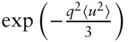, where 〈 u 2〉 is the mean‐squared displacement from the scattering centre.

For a sample with quasi‐long‐range order, the scattering profile consists of a sharp peak with power‐law tails ( Figure 1.10b). More commonly observed is short‐range order. This produces a scattering profile containing a Lorentzian peak ( Figure 1.10c) given by

(1.57)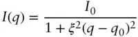

Here ξ is a correlation length and q 0= 2π/d is the peak position ( d is the preferred spacing in the system). If the decay of the peaks in the correlation function is steeper, g ( r ) ∼ exp(− r 2/ ξ 2), then the intensity profile shows a Gaussian peak:

(1.58)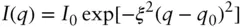

For more ordered or partly crystalline materials, paracrystal models can be employed in the analysis of SAS data. Paracrystals are imperfect crystals in which a degree of lattice order is retained. Figure 1.11illustrates paracrystals of the first and second kind, for the case of a two‐dimensional lattice.

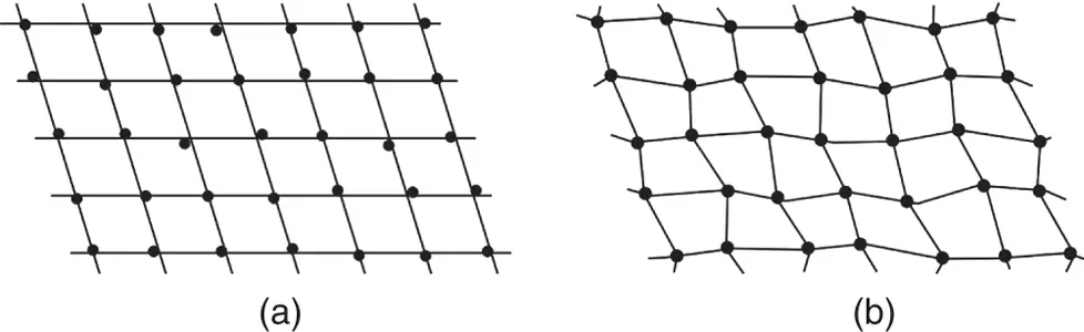
Figure 1.11 Schematic of lattice distortions in paracrystals with lattice distortions of (a) first and (b) second kind.

In a paracrystal with imperfections of the first kind, the long‐range lattice order is retained but there are fluctuations in position around the lattice nodes ( Figure 1.11a), i.e. there is positional disorder. In the observed diffraction pattern, the peak width increases linearly with the peak order [31], and the intensity is modulated by a Debye‐Waller factor as described above [12, 31]. With lattice distortions of the second kind, the long‐range lattice order is disrupted as shown in Figure 1.11b, i.e. there is long‐range positional and bond orientational disorder. This leads to a quadratic increase in peak width with peak order [12, 31]. Analytical solutions are available for one‐dimensional paracrystal models of the first and second kind [12, 22].

The amplitude structure factor in Eq. (1.27)is a complex quantity and so can be written as the product of an amplitude and a phase:

( 1.59)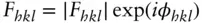

where ϕhkl is the phase angle for reflection with indices hkl . The amplitude can be obtained from the square root of the intensity:

(1.60)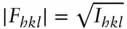

In general, the phase appearing in Eq. (1.59)cannot be determined in an x‐ray diffraction or SAXS experiment. There are methods in x‐ray crystallography to circumvent the problem (such as heavy atom replacement). In the study of SAXS by soft materials, the reconstruction of the electron density profile is usually only done for a limited subset of systems. In particular, it is performed for lamellar structures such as those of lipid bilayers, as discussed further in Section 4.12.

A number of structure factors have been proposed for fractal structures. For these systems, the separation of form and structure factors often does not make sense; therefore, we denote the scattering just by the intensity. One model commonly used in the analysis of SAS data is the Fischer–Burford fractal model, for which the structure factor is given by [32, 33]

(1.61)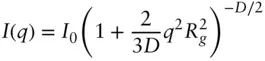

where I 0is the forward scattering intensity, D is the fractal dimension, and Rg is the radius of gyration of the aggregate.

Another widely employed expression is that for the structure factor of a mass‐fractal: [33–36]

(1.62)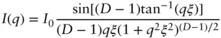

where I 0denotes forward scattering, D is the fractal dimension, and ξ is the correlation length.

Another widely used model was developed by Beaucage for a variety of systems with ordering on multiple length scales including fractal structures, and is based on an expression for the scattering from excluded volume polymer fractals [37, 38]. This gives a function that interpolates between a Guinier function at low q and a Porod function at high q . It is used for many types of systems, such as porous materials ( Section 5.11), colloidal and gel aggregate structures, polymer foams, polymer nanocomposites, nanopowders, and other systems. The unified Beaucage expression for a system with one structural level is [39]:

( 1.63)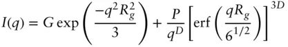

Here G is a Guinier scaling factor, Rg is the radius of gyration of the mass fractal object, P is a Porod constant, D is the fractal dimension, and erf denotes the error function. The constant P is related to G via the expression [38]:

( 1.64)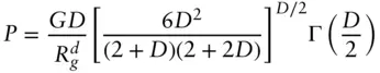

Here Γ( D /2) denotes a Gamma function. Analytical expressions are available for G and P for a variety of uniform particles with different shapes as well as types of polymers [40].

Figure 1.12shows an example of a fit to USAXS data for a titania nanopowder, along with indicated contributions from the Guinier and Porod components of Eq. (1.64).

Figure 1.12 Example of fitting of SAS data using the unified Beaucage model, Eq. (1.63), to fit USAXS data for a titania nanopowder (inset: TEM image). The contributions from the Guinier and Porod components of Eq. (1.63)are shown. Also shown for comparison is the limiting Porod slope in a scattering profile from spheres of the same radius of gyration Rg as from the Beaucage model fit.

Source : From Beaucage et al. [40]. © 2004, International Union of Crystallography.