Ian W. Hamley - Small-Angle Scattering

(1.47)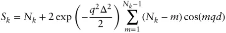

In the second model, the paracrystalline model (this type of model is discussed further in Section 1.6.3), the position of an individual fluctuating layer in a paracrystal is determined solely by its nearest neighbours. Then [21, 22]

(1.48)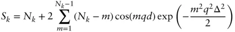

In a third alternative model, introduced by Caillé [23] and modified to allow for finite lamellar stacks [24, 25], the fluctuations are quantified in terms of the flexibility of the membranes:

(1.49)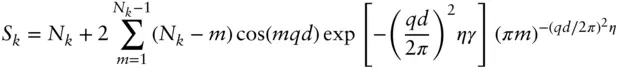

Here γ is Euler's constant and

(1.50)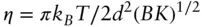

is the Caillé parameter, which depends on the bulk compression modulus B and the bending rigidity K of the layers.

For ordered systems such as colloid crystals, liquid crystals or block copolymer mesophases, the structure factor will comprise a series of Bragg reflections (or pseudo‐Bragg reflections, strictly, for layered structures). The amplitude structure factor for a hkl reflection (where h, k and l are Miller indices) of a lattice is given by [12]

( 1.51)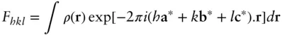

Here a*, b*, and c* are reciprocal space axis vectors. In Eq. (1.51), ρ ( r) is used rather than Δ ρ ( r) since if Fhkl is determined on an absolute scale, the Fourier transform of Eq. (1.51)permits the determination of ρ ( r) in absolute units (e.g. electron Å −3in the case of SAXS data).

The location of the observed Bragg reflections (ratio of peak positions) is characteristic of the symmetry of the structure. Table 1.1lists the observed reflections for common structures observed for soft materials (and some hard materials). Figure 1.7shows examples of structures with the lowest indexed planes indicated. The generating equations for allowed reflections for different space groups are available in crystallography textbooks [26] and elsewhere [27].

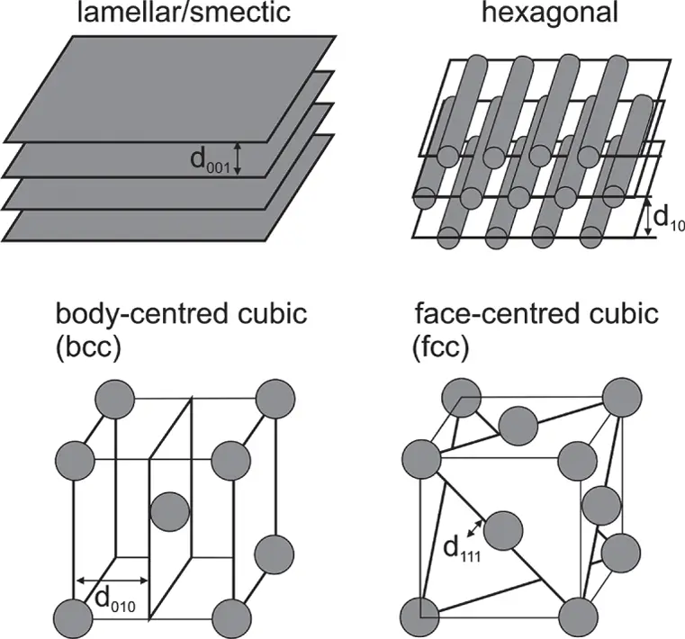
Figure 1.7 Representative one‐, two‐, and three‐dimensional structures, with lowest indexed diffraction planes indicated. For the lamellar structure, three‐dimensional Miller indices have been employed while for the hexagonal structure two‐dimensional indices are used.

Figure 1.8shows representative SAXS intensity profiles for some common ordered phases in soft materials, exemplified by data for block copolymer melts. The sequences of observed reflections are consistent with Table 1.1.

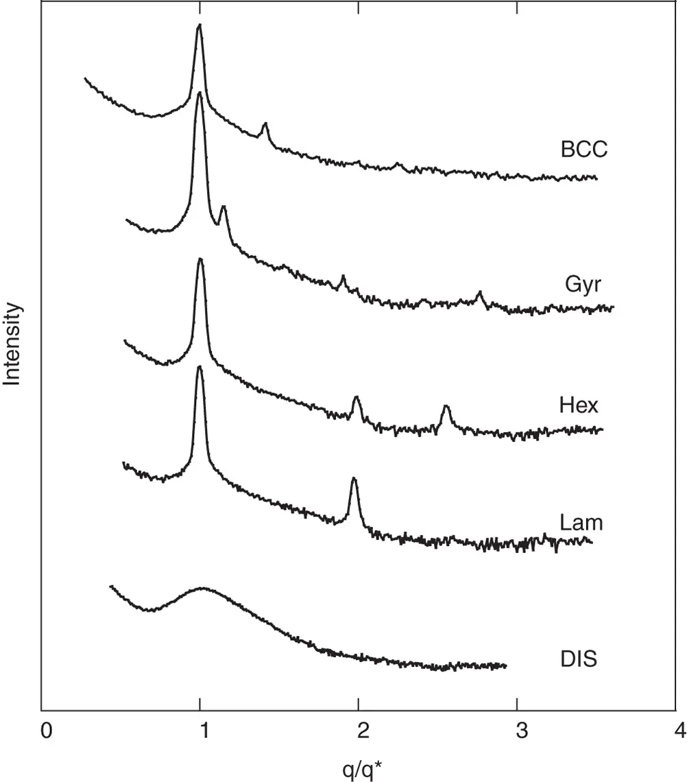
Figure 1.8 Compilation of SAXS profiles measured for PEO‐PBO [polyoxyethylene‐ b ‐polyoxybutylene] diblock copolymer melts. The x ‐axis uses a q ‐scale normalized to q *, the position of the first order peak. BCC: body‐centred cubic, Gyr: gyroid, Hex: hexagonal‐packed cylinders, Lam: lamellar, DIS: disordered.

Source : From Ref. [28].

The layer spacing d for a lamellar phase is given by

( 1.52)

Here q lis the position of the l th order Bragg peak.

For a two‐dimensional hexagonal structure [26, 29]:

( 1.53)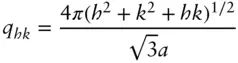

where qhk is the position of the Bragg peak with indices hk and a is the lattice constant.

For a cubic structure [26, 29]

( 1.54)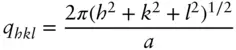

where qhkl is the position of the Bragg peak with indices hkl and a is the lattice constant.

The general expression for all crystal systems is [12, 26]

(1.55)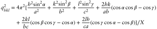

with

(1.56)

Here a , b , c are the unit cell lengths and α , β , γ are the unit cell angles.

Explicit expressions for qhkl for other lattices can be found elsewhere (see e.g. [26, 29]). Figure 1.9shows an example of the determination of the lattice constant a by use of Eq. (1.54)by indexing the observed reflections of a cubic structure (lipid bicontinuous cubic structure). Similar methods can be used to determine d for lamellar structures from Eq. (1.52)or a for hexagonal structures from Eq. (1.53).

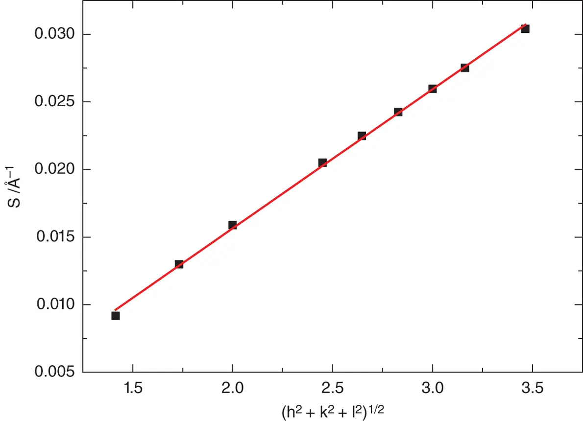
Figure 1.9 Indexation of SAXS reflections observed for the lipid monoolein forming a bicontinuous cubic structure, within cubosomes. Here, S hkl= 1/ d hklis determined from the observed position of the reflection via S hkl= q hkl/2π. The lattice constant a = (97.2 ± 1.2) Å is determined as the reciprocal of the gradient.

Source : From Ref. [15].

The number of observed reflections as well as the peak width for an ordered structure gives an indication of the extent of order. Figure 1.10illustrates this schematically for a one‐dimensional lattice with variable degrees of short‐ or long‐ranged order [20, 30].

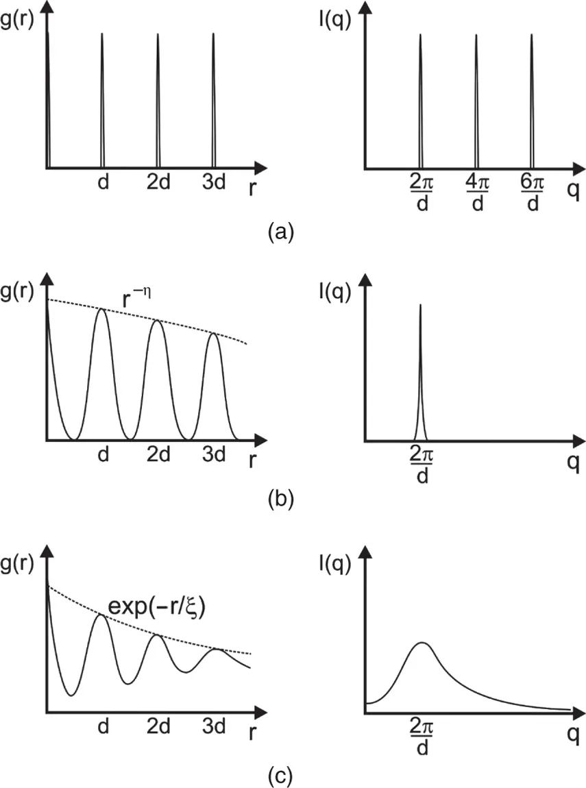
Figure 1.10 Long‐range versus short‐range order showing schematics of real space distribution functions g ( r ) (left), and scattered intensity profiles I ( q ) (right). (a) Long-range order, (b) Quasi-long-range order, (c) Short range order.