Barna Szabó - Finite Element Analysis

When the exact solution is an analytic function then 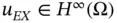and the asymptotic rate of convergence is exponential:

(1.93)

where C , γ and θ are positive constants, independent of N . In one dimension , in two dimensions , in three dimensions , see [10].

When the exact solution is a piecewise analytic function then eq. (1.93)still holds provided that the boundary points of analytic functions are nodal points, or more generally, lie on the boundaries of finite elements.

The relationship between the error 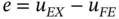measured in energy norm and the error in potential energy is established by the following theorem.

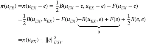
Theorem 1.5

(1.94)

Proof: Writing and noting that , from the definition of we have:

Remark 1.10Consider the problem given by eq. (1.5)and assume that κ and c are constants. In this case the smoothness of u depends only on the smoothness of f : If then for any . Similarly, if then for any . This is known as the shift theorem. More generally, the smoothness of u depends on the smoothness of κ , c and F . For a precise statement and proof of the shift theorem we refer to [21].

Remark 1.11An introductory discussion on how a priori estimates are obtained under the assumption that the second derivative of the exact solution is bounded can be found in Appendix B.

The goal of finite element computations is to estimate certain quantities of interest (QoIs) such as, for example, the maximum and minimum values of u or on . Since finite element solutions are approximations to an exact solution, it is not sufficient to report the value of a QoI computed from the finite element solution. It is also necessary to provide an estimate of the relative error in the QoI, or present evidence that the relative error in the QoI is not greater than an acceptable value.

In this section we will use the a priori estimates described in Section 1.5.2to obtain a posteriori estimates of error in energy norm. It is possible to obtain very accurate estimates for a large class of problems which includes most problems of practical interest.

For most practical problems the estimate (1.92)is sufficiently sharp so that the less than or equal sign (≤) can be replaced by the approximately equal sign (≈) and this a priori estimate can be used in an a posteriori fashion.

The computed values of the potential energy corresponding to a sequence of finite element spaces can be used for estimating the error in energy norm by extrapolation. Sequences of finite element spaces that have this property are called hierarchic sequences. By Theorem 1.5and eq. (1.92)we have:

(1.95)

where . There are three unknowns: , and β . Assume that we have a sequence of solutions corresponding to the hierarchic sequence of finite element spaces . Let us denote the corresponding computed potential energy values by , , πi and the degrees of freedom by , , Ni . We will denote the estimate for by π∞ . With this notation we have: