Edoardo Provenzi - From Euclidean to Hilbert Spaces

This holds for any j ∈ {1, . . . , n }, so the orthogonal family F is free.□

Using the general theory of vector spaces in finite dimensions, an immediate corollary can be derived from theorem 1.10.

COROLLARY 1.1.– An orthogonal family of n non-null vectors in a space ( V , 〈, 〉) of dimension n is a basis of V .

DEFINITION 1.6.– A family of n non-null orthogonal vectors in a vector space ( V , 〈, 〉) of dimension n is said to be an orthogonal basis of V . If this family is also orthonormal, it is said to be an orthonormal basis of V .

The extension of the orthogonal basis concept to inner product spaces of infinite dimensions will be discussed in Chapter 5. For the moment, it is important to note that an orthogonal basis is made up of the maximum number of mutually orthogonal vectors in a vector space . Taking n to represent the dimension of the space V and proceeding by reductio ad absurdum, imagine the existence of another vector u *∈ V , u ≠ 0, orthogonal to all of the vectors in an orthogonal basis ; in this case, the set would be free as orthogonal vectors are linearly independent, and the dimension of V would be n + 1 instead of n ! This property is usually expressed by saying that an orthogonal family is a basis if it is not a subset of another orthogonal family of vectors in V .

Note that in order to determine the components of a vector in relation to an arbitrary basis, we must solve a linear system of n equations with n unknown variables. In fact, if v ∈ V is any vector and ( u i) i = 1, . . . , n is a basis of V , then the components of v in ( u i) are the scalars α 1, . . . , α nsuch that:

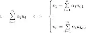
where u i,jis the j -th component of vector u i.

However, in the presence of an orthogonal or orthonormal basis, components are determined by inner products, as seen in Theorem 1.11.

Note, too, that solving a linear system of n equations with n unknown variables generally involves far more operations than the calculation of inner products; this highlights one advantage of having an orthogonal basis for a vector space.

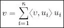
THEOREM 1.11.– Let B = { u 1, . . . , u n} be an orthogonal basis of ( V , 〈, 〉). Then:

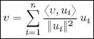
Notably, if B is an orthonormal basis, then:

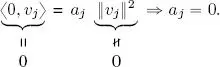
PROOF.– B is a basis, so there exists a set of scalars α 1, . . . , α nsuch that . Consider the inner product of this expression of v with a fixed vector u i, i ∈ {1, . . . , n }:

so 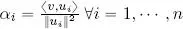, and thus 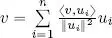. If B is an orthonormal basis, ‖ u i‖ = 1 giving the second law in the theorem.□

Geometric interpretation of the theorem: The theorem that we are about to demonstrate is the generalization of the decomposition theorem of a vector in plane ℝ 2or in space ℝ 3on a canonical basis of unit vectors on axes. To simplify this, consider the case of ℝ 2.

If and are, respectively, the unit vectors of axes x and y , then the decomposition theorem says that:

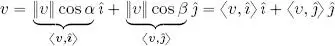
which is a particular case of the theorem above.

We will see that the Fourier series can be viewed as a further generalization of the decomposition theorem on an orthogonal or orthonormal basis.

The definition of orthogonal projection can be extended by examining the geometric and algebraic properties of this operation in ℝ 2and ℝ 3. Let us begin with ℝ 2.

In the Euclidean space ℝ 2, the inner product of a vector v and a unit vector evidently gives us the orthogonal projection of v in the direction defined by this vector, as shown in Figure 1.2with an orthogonal projection along the x axis.

The properties verified by this projection are as follows:

1) projecting onto the x axis a second time, vector P x v obviously remains unchanged given that it is already on the x axis, i.e. . Put differently, the operator P xbound to the x axis is the identity of this axis;

2) the difference vector between v and its projection v − P x v is orthogonal to the x axis, as we see from Figure 1.3;

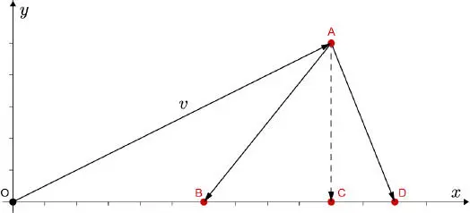
Figure 1.2. Orthogonal projection and diagonal projections and of a vector in v ∈ ℝ 2 onto the x axis. For a color version of this figure, see www.iste.co.uk/provenzi/spaces.zip