Edoardo Provenzi - From Euclidean to Hilbert Spaces

The theorem demonstrated above tells us that the vector in the vector subspace S ⊆ V which is the most “similar” to v ∈ V (in the sense of the norm induced by the inner product) is given by the orthogonal projection. The generalization of this result to infinite-dimensional Hilbert spaces will be discussed in Chapter 5.

As already seen for the projection operator in ℝ 2and ℝ 3, the non-negative scalar quantity gives a measure of the importance of in the reconstruction of the best approximation of v in S via the formula 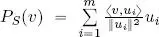: if this quantity is large, then is very important to reconstruct P S( v ), otherwise, in some circumstances, it may be ignored. In the applications to signal compression, a usual strategy consists of reordering the summation that defines P S( v ) in descent order of the quantities and trying to eliminate as many small terms as possible without degrading the signal quality.

This observation is crucial to understanding the significance of the Fourier decomposition, which will be examined in both discrete and continuous contexts in the following chapters.

Finally, note that the seemingly trivial equation v = v − s + s is, in fact, far more meaningful than it first appears when we know that s ∈ S : in this case, we know that v − s and s are orthogonal.

The decomposition of a vector as the sum of a component belonging to a subspace S and a component belonging to its orthogonal is known as the orthogonal projection theorem .

This decomposition is unique, and its generalization for infinite dimensions, alongside its consequences for the geometric structure of Hilbert spaces, will be examine in detail in Chapter 5.

As we have seen, projection and decomposition laws are much simpler when an orthonormal basis is available.

Theorem 1.13 states that in a finite-dimensional inner product space, an orthonormal basis can always be constructed from a free family of generators.

THEOREM 1.13.– (The iterative Gram-Schmidt process 6) If ( v 1, . . . , v n), n ≼ ∞ is a basis of ( V , 〈, 〉), then an orthonormal basis of ( V , 〈, 〉) can be obtained from ( v 1, . . . , v n).

PROOF.– This proof is constructive in that it provides the method used to construct an orthonormal basis from any arbitrary basis.

– Step 1: normalization of v 1:

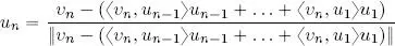
– Step 2, illustrated in Figure 1.5: v 2is projected in the direction of u 1, that is, we consider 〈 v 2, u 1〉 u 1. We know from theorem 1.12 that the vector difference v 2− 〈 v 2, u 1〉 u 1is orthogonal to u 1. The result is then normalized:

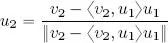
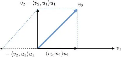
Figure 1.5. Illustration of the second step in the Gram-Schmidt orthonormalization process. For a color version of this figure, see www.iste.co.uk/provenzi/spaces.zip

– Step n , by iteration:

The most important properties of an orthonormal basis are listed in theorem 1.14.

THEOREM 1.14.– Let ( u 1, . . . , u n) be an orthonormal basis of ( V , 〈, 〉), dim ( V ) = n. Then , ∀ v, w ∈ V :

1) Decomposition theorem on an orthonormal basis :

[1.7]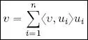

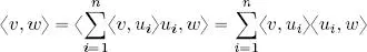
2) Parseval’s identity 7 :

[1.8]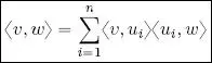

3) Plancherel’s theorem 8 :

[1.9]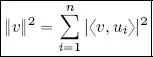

Proof of 1 : an immediate consequence of Theorem 1.12. Given that ( u 1, . . . , u n) is a basis, v ∈ span( u 1, . . . , u n); furthermore, ( u 1, . . . , u n) is orthonormal, so 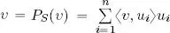. It is not necessary to divide by ‖ u i‖ 2when summing since ‖ u i‖ = 1 ∀ i .

Proof of 2 : using point 1 it is possible to write 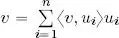, and calculating the inner product of v , written in this way, and w , using equation [ 1.1], we obtain:

Proof of 3 : writing w = v on the left-hand side of Parseval’s identity gives us 〈 v, v 〉 = ‖ v ‖ 2. On the right-hand side, we have:

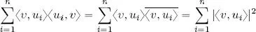
hence .

NOTE.–

1) The physical interpretation of Plancherel’s theorem is as follows: the energy of v , measured as the square of the norm, can be decomposed using the sum of the squared moduli of each projection of v on the n directions of the orthonormal basis ( u 1, ..., u n).

In Fourier theory, the directions of the orthonormal basis are fundamental harmonics (sines and cosines with defined frequencies): this is why Fourier analysis may be referred to as harmonic analysis .