Scott D. Sudhoff - Power Magnetic Devices

The next step in the design process is to determine the parameter space Ω. This is tabulated in Table 1.7. Some level of engineering estimation is required to select a reasonable range. However, situations where a range is incorrectly set are usually easy to detect by looking at the population distribution. We will return to this point.

We have now set forth a fitness function and a domain for the parameter vector, and so we can proceed to conduct an optimization. We will begin with a single‐objective case. To conduct this study, a MATLAB‐based genetic optimization toolbox known as GOSET was used. This open‐source code and the code for this particular example are available at no cost in Sudhoff [6].

Figure 1.23illustrates the progression of the study, which was conducted with a population size of 1000 over 1000 generations. Therein, Figure 1.23(a) shows the gene distribution at the end of the optimization. Recall that θ iis the normalized value of the i th gene. Each design is shown in encoded parameter space as a series of dots, each with its own shade (for example, a certain dark shade may correspond to design 37 of the population). Because of the large numbers of designs, it is not possible to pick one design among all the designs. However, a sense of the distribution of the gene (parameter) values in the population can readily be obtained. The horizontal coordinate of each design within its parameter window is proportional to its ranked fitness—with lower ranks toward the left side of the window for a given parameter and higher ranks toward the right side of a given window. Considerable information can be discerned from the distribution plot. For example, there seems to be more sensitivity to d s(which is tightly clustered) than to w s(which is less tightly clustered). A distribution of a gene (parameter) value at the bottom or top of the range indicates that it may be appropriate to adjust the domain of that parameter.

Figure 1.23(b) depicts the fitness versus generation. The best fitness in the population, the median fitness of the population, and the mean fitness of the population are shown. Note that for a few generations, the best fitness is zero (actually slightly < 0), but then the best fitness increases rapidly until generation 150 or so, after which the fitness climes more slowly. The median and mean fitness rise more slowly than the fitness of the best individual. Observe that there are large rapid changes in the median fitness because this is a fitness of the median individual which changes from generation to generation. The mean fitness of the population is more stable. As can be seen, the mean fitness of the population occasionally goes down; this does not happen in the case of the fitness of the most fit individual in the population because of the elitism operator.

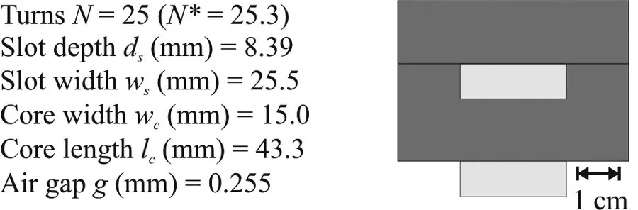
Figure 1.24 UI‐core design.

The most fit individual in the final population is illustrated in Figure 1.24, which lists the design parameters as well as a cross‐sectional diagram. Note that N *= 25.3 maps to N = 25 from (1.10-2). The design’s mass is 0.578 kg, and the power loss at rated current is W. The inductance is right at 1 mH and the flux density is at 0.617 T. The current density of the design is 1.67 A/mm 2. It would appear that our design is against all constraint limits except those on mass and current density.

At this point, the question arises regarding how we know that our design is optimal. Unfortunately, we do not. There is not an optimization algorithm known that can guarantee convergence to the global optimum for a generic problem without known mathematical properties. However, in the GOSET code used for this example, a traditional optimization method (Nelder–Mead simplex) is used to optimize the design starting from the endpoint of the GA run, and this helps to ensure a local optimum. Still, there is no guarantee that a global optimum is obtained. Therefore, the prudent designer will re‐run the optimization several times in order to gain confidence in the results. The runs can then be inspected to see if all runs converged to the same fitness. If significant variation in fitness has occurred, the use of more generations and/or a larger population size is indicated.

For our single‐objective optimization problem, the optimization was re‐run a multitude of times in order to investigate the variability of the design obtained from one run to the next. We will view variation of parameters and metrics in terms of normalized standard deviations. For example, the normalized standard deviation of the number of turns is the standard deviation of the number of turns divided by the median value of the number of turns for each design, interpreted as a percentage. Conducting the optimization process 100 times yielded the following normalized standard deviations: N with a 11%, d swith a 4.4%, w swith a 17%, w cwith a 6.4%, l cwith a 14%, and g with a 11% standard deviation. These may seem relatively large. However, it is interesting that normalized standard deviation in mass is only 1.0%. This indicates that there is a family of designs with equally good performance. It is interesting to observe that while appreciable design variation was found, every solution determined was viable (and not that different in terms of performance metrics).

It may seem objectionable to the reader that the results are not repeatable, which arises from the use of a random set of initial designs, and stochastic operators in the GA. However, even Newton’s method will generate random variation in the solution of an optimization problem if the initial condition is selected at random. In Newton’s method, providing a consistent initial condition will of course produce a consistent final answer; however, being consistent can merely mean being consistently incorrect—which can happen if the algorithm becomes consistently trapped at a same local minimizer while missing the global minimizer.

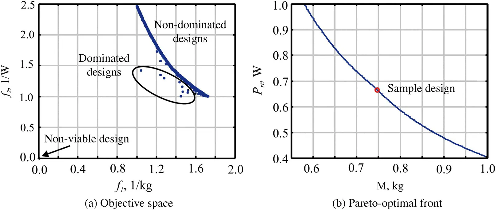
Figure 1.25 Multi‐objective optimization results.

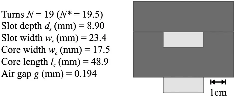
Figure 1.26 Sample design from Pareto‐optimal front.

Let us now turn our attention to a multi‐objective optimization of the UI‐core inductor. The only change in our approach is the replacement of (1.10-14)by (1.10-15). Using 2000 generations with a population size of 1000 yields the results shown in Figure 1.25. Figure 1.25(a) illustrates the objective space at the end of the optimization run. Each point in Figure 1.25(a) represents the objectives of a complete design. Nonviable designs have fitness values close to the origin (and are slightly negative in each axis). Viable, but dominated, designs are also apparent. The remaining designs are nondominated. In Figure 1.25(b) only the nondominated designs are shown, and the fitness elements are reciprocated so that mass and loss can be plotted directly. Again, each point represents the mass and loss of an individual design. Note the tradeoff between mass and loss. This will be a recurrent theme in this text. A sample design on the front is also indicated; this design is illustrated in more detail in Figure 1.26. The sample design has a mass of 0.75 kg, and a loss at rated current of 0.67 W. The inductance is just over 1 mH, and flux density at rated current is 0.617 T. The current density at rated current is 1.3 A/mm 2.