Scott D. Sudhoff - Power Magnetic Devices

In order to illustrate this algorithm, let us apply Kung’s algorithm to the set of designs illustrated in Figure 1.15. For this problem, P= {1, 2, 3, 4, 5, 6, 7, 8}. Considering cost to be our first objective, P s= {1, 6, 2, 3, 8, 4, 7, 5}. Figure 1.18illustrates the calls to the front routine. Therein, the order of the calls and the input and output arguments to each call are indicated. The basis of this method is that whenever the front is called, its return argument Rwill never have any dominated members. This is a result of the following: (a) The sorting of the first objective ensures that no member of a return argument Tcan be dominated by a member of B, (b) every member of Bis checked against every member of Tbefore returning to the next higher level, and (c) a set of one is inherently a nondominated set. As a result, T, B, and Rare all nondominated sets.

In executing this example, calls 4, 5, 7, 8, 11, 12, 14, and 15 return nondominated sets because their input and output argument set size is 1. In calls 3, 6, 10, and 13, no member of an input set Tcan be dominated by the corresponding set Bbecause of the ordering with respect to the first objective. The return arguments of calls 3, 6, 10, and 13 cannot have dominated members because the input sets to these calls ( Tand B) were nondominated, no member of Tcan be dominated by a member of B, and every member of Bis checked against every member of T. Thus, proceeding from the bottom of Figure 1.18to the top as subroutine calls are made, we see that the process involves a gradual combining and sifting of smaller nondominated sets to yield a larger nondominated set.

One question that arises in this example is why we need function calls beyond call 1 as it generates the nondominated set. It must be remembered that the calls are recursive in nature and so the algorithm of call 1 cannot be completed without calls 2–15. Another question that is often asked is if we really need to make calls to front when the number of elements in the input set is one. With some additional if‐then constructs, calls to front with an input set size of one could in fact be avoided.

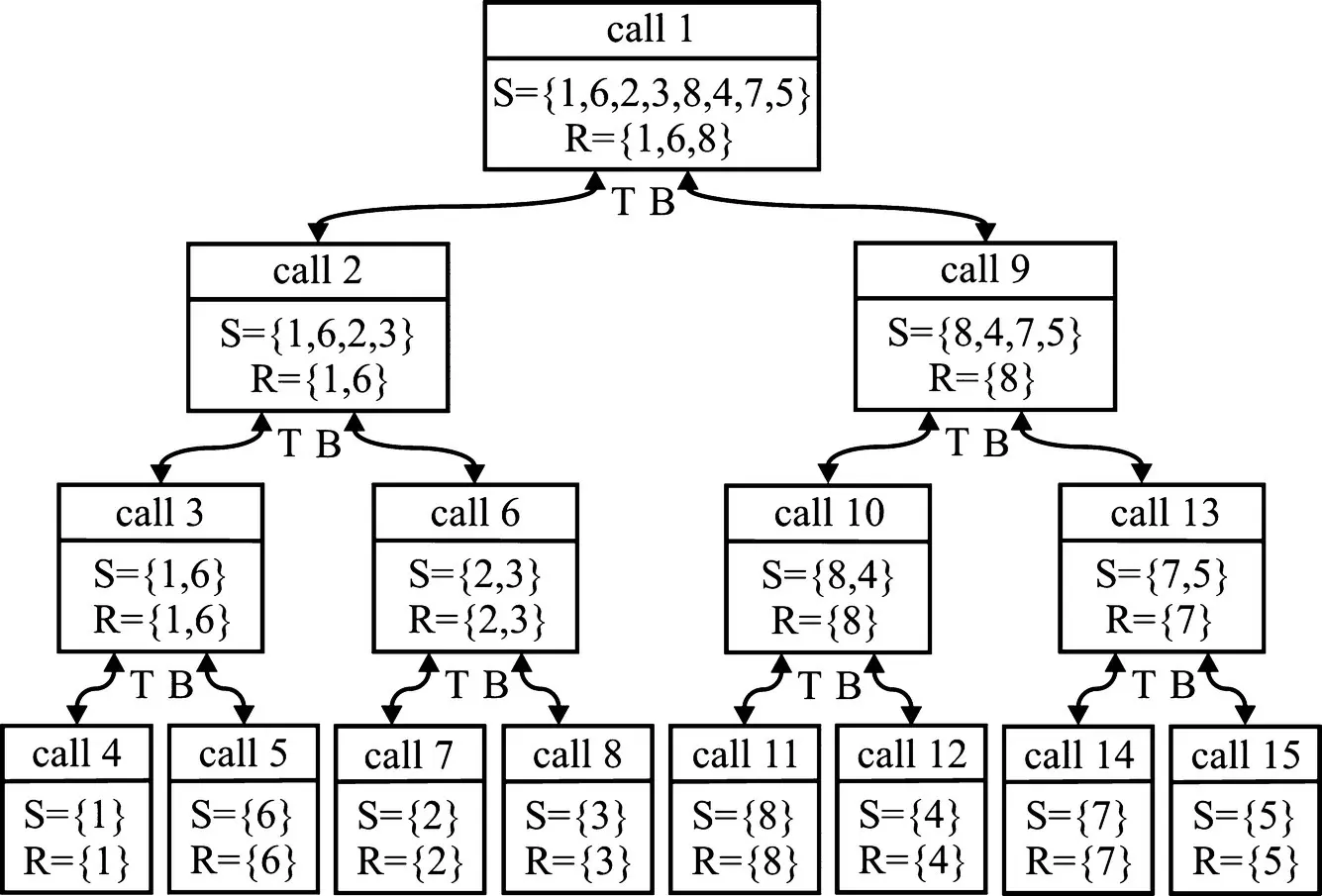
Figure 1.18 Application of Kung’s method.

In addition to Kung’s method, two more processes will be needed in order to set forth the elitist NSGA‐II. The first of these is nondominated sorting (NDS). In order to understand NDS, let us consider again Figure 1.15with population P= {1, 2, 3, 4, 5, 6, 7, 8}. As we have already discussed, the nondominated set is {1,6,8}, which was found using Kung’s algorithm. Let us consider this set front 1, denoted F 1. Now suppose we remove the members of F 1from P, and find the nondominated set of the remaining population by again applying Kung’s algorithm. This will yield the second front, given by F 2= {2, 3, 7}. Now let us once more consider the population Pbut now less the members in F 1and F 2. Finding the nondominated set of the remaining population by again applying Kung’s algorithm yields the third front, F 3= {4, 5}. In this way, it is possible to associate with every member of the population a rank with regard to which front they are associated. This ranking will be used to compare different members of the population in order to determine which members will become a part of the mating pool.

Although a population member on the first front can be said to be superior to a member on the second front, the question arises as to how to compare solutions on the same front. This issue will be resolved using the concept of crowding distance. The crowding distance associated with a solution x iis defined as

(1.8-2)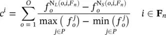

where F nis the set of indices in front n , we assume i is in front F n, o is an index of objective number, O is the number of objectives, N L( o , i , F n) returns the index of the individual with the next largest fitness (greater than individual i ) in the o th objective in front F n, and N S( o , i , F n) returns the index of the individual with the next smallest fitness (less than individual i ) in the o th objective in front F n. In the case where there is no next larger or smaller individual in some objective—that is, it is a maximum or minimum in some objective—the crowding distance is taken as a very large number (pseudo‐infinity).

Crowding tournament selection uses the concepts of front rank and crowding distance in order to decide which individuals to put into the mating pool. In this method, individuals x c1and x c2are randomly drawn from the current population. If one of these solutions has a better front rank than the other, it is copied into a mating pool. If the two individuals have the same front rank, then the one with the better (larger) crowding distance goes into the mating pool, as it has greater diversity in terms of objectives.

The concept of crowding distance is illustrated in Figure 1.19. Suppose we wish to calculate the crowding distance of population member 7. Using (1.8-2), we have

(1.8A-1)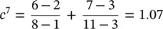

At this point, the remaining elements of the NSGA‐II can be set forth. The process is illustrated in Figure 1.20. Therein, we start with a population P[ k ]. Using crowded tournament selection (CTS), a mating pool Mis created which is in turn used to create a population of children C. Next, the current population P[ k ] is combined with the children Cto form an enlarged population R. Non NDS is used to divide this population into groups based on front, yielding sets F 1, F 2, and so on. Next, these sets are used to create the next generation P[ k + 1]. This is done by filling P[ k + 1]with sets of fronts from first to last. At some point, shown as F 3in Figure 1.20, the full front will have more members than remain empty in P[ k + 1]. At this point, crowding distance selection (CDS) is used to determine which members of the final included front are included in P[ k + 1]. In particular, the members of F 3with the best crowding distance are used to complete the next population.

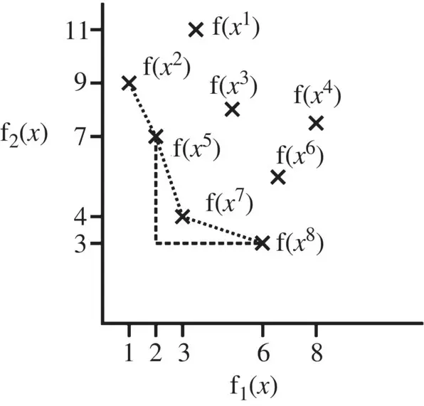
Figure 1.19 Crowding distance.

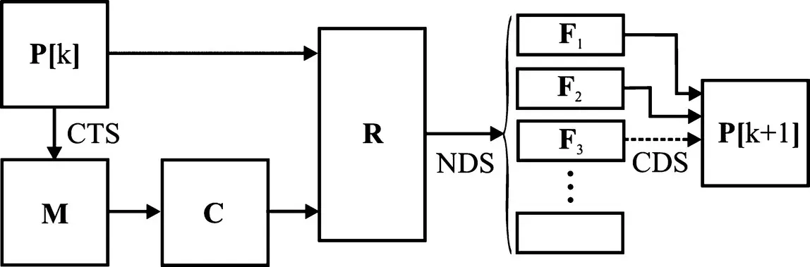
Figure 1.20 Elitist nondominated sorting genetic algorithm (NSGA‐II).