Scott D. Sudhoff - Power Magnetic Devices

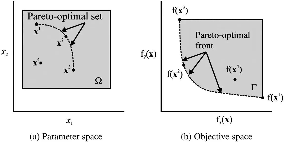
Figure 1.16 Pareto‐optimal set and front.

The concepts of a Pareto‐optimal set and Pareto‐optimal front are illustrated in Figure 1.16for a system with a two‐dimensional parameter space (i.e., a two‐dimensional parameter vector) and a two‐dimensional objective space. As an example, if we were designing an inductor, the variables of the parameter space may consist of the number of turns and diameter of the wire, variables in the objective space might be inductor volume and inductor power loss. Returning to Figure 1.16(a) we see the parameter space defined over a set Ω (shaded). Members of this set include x 1, x 2, x 3, and x 4 .Every point in Ω is mapped to a point in objective space Γ (also shaded) shown in Figure 1.16(b). For example, x 4in parameter space maps to f( x 4) in objective space. Points along the dashed line in Ωin Figure 1.16(a) are nondominated and form the Pareto‐optimal set. They map to the dashed line in Figure 1.16(b) in objective space where they form the Pareto‐optimal front.

The goal of multi‐objective optimization is to calculate the Pareto‐optimal set and the associated Pareto‐optimal front. One may argue that in the end, only one design is chosen for a given application. This is often the case. However, to make such a decision requires knowledge of what the tradeoff between competing objectives is—that is, the Pareto‐optimal front.

There are many approaches to calculating the Pareto‐optimal set and the Pareto‐optimal front. These approaches include the weighted sum method, the ε ‐constraint method, and the weighted metric method, to name a few [10]. In each of these methods, the multi‐objective problem is converted to a single‐objective optimization, and that optimization is conducted to yield a single point on the Pareto‐optimal front. Repetition of the procedure while varying the appropriate parameters yields the Pareto‐optimal front.

In order to illustrate this procedure, let us consider the ε ‐constraint method for a system with two objectives, f 1( x) and f 2( x), which we wish to minimize. In order to determine the Pareto‐optimal set and front, the problem

(1.7-1)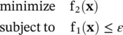

is repeatedly solved for different values of ε . This minimization can be carried out numerically using any single‐objective minimization method. Solving (1.7-1)with ε = ε 1ayields x 1awith objective function values ( ε 1a,f 2( x 1a)) which is a point on the Pareto‐optimal front, as shown in Figure 1.17. Solving (1.7‐2) with ε = ε 1byields x 1bwith objective function values ( ε 1b,f 2( x 1b)). Repeating the procedure over a range of ε values, the Pareto‐optimal set and front can be determined.

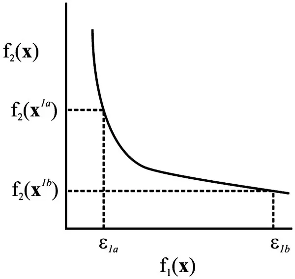
Figure 1.17 Calculation of Pareto‐optimal front with ε‐constraint method.

In more concrete terms, suppose we wished to minimize volume and loss for some electromagnetic device. If our first objective was volume and our second objective was loss, we would repeatedly minimize loss with different constraints on the volume. In this case, each ε value would correspond to a different volume. For each numerically different volume constraint, we would get the corresponding loss and thereby—one single‐objective optimization at a time—build up a Pareto‐optimal front between volume and loss.

As it turns out, GAs are well‐suited to compute Pareto‐optimal sets. This is because they operate on a population. In multi‐objective optimizations, the population of designs can be made to conform to the Pareto‐optimal set. This allows a GA to determine the Pareto‐optimal set and Pareto‐optimal front in a single analysis without requiring the solution of a separate optimization for every point on the front as is needed in the weighted sum method, ε ‐constraint method, and weighted metric methods.

GAs are well‐suited for multi‐objective optimization, and there are a large number of approaches that can be taken. The goal in all of these methods is to evolve the population so that it becomes a Pareto‐optimal set.

Multi‐objective GAs fall into two classes, nonelitist and elitist. The elitist strategies are particularly effective because they explicitly identify and preserve, when possible, the nondominated individuals. Elitist strategies include the elitist nondominated sorting GA (NSGA‐II), distance‐based Pareto GA, and the strength Pareto GA [11]. In order to keep the present discussion limited that we might soon start discussing device design, we will somewhat arbitrarily focus our attention on the elitist NSGA‐II.

Before setting forth this algorithm, we will first consider the problem of finding the nondominated individuals in a population. Since finding the Pareto‐optimal front is the goal of any multi‐objective optimization, being able to identify those candidate solutions which are nondominated will be an important task. In a generic sense, the nondominated solutions will be given a favored status in many multi‐objective methods. To identify the nondominated solutions, we will consider Kung’s method. Consider a population P. We wish to find the nondominated subset of P ,which we will denote E. The first step in Kung’s method is to sort the members of Pfrom best to worst in terms of the first objective. In the event that two or more members have identical values of the first objective, this subset is ordered by the second objective (and by subsequent objectives if necessary). This sorted population will be denoted P s. The nondominated set Eis then calculated as

Table 1.5 Pseudo‐Code for Kung’s Method

(1.8-1)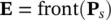

where front() is a recursively defined function. In order to describe this function, let ∣ · ∣ denote the number of elements in a set, and let P a:bdenote the a th to b th individuals in a population or set. With this notation, the pseudo‐code for Kung’s algorithm is listed in Table 1.5. Therein, Sand Rdenote the input and output of the routine. The terms T, B, and Nrefer to intermediate variables that represent sets. The variable i is a scalar integer index.