Scott D. Sudhoff - Power Magnetic Devices
Здесь есть возможность читать онлайн «Scott D. Sudhoff - Power Magnetic Devices» — ознакомительный отрывок электронной книги совершенно бесплатно, а после прочтения отрывка купить полную версию. В некоторых случаях можно слушать аудио, скачать через торрент в формате fb2 и присутствует краткое содержание. Жанр: unrecognised, на английском языке. Описание произведения, (предисловие) а так же отзывы посетителей доступны на портале библиотеки ЛибКат.
- Название:Power Magnetic Devices
- Автор:
- Жанр:
- Год:неизвестен
- ISBN:нет данных
- Рейтинг книги:4 / 5. Голосов: 1
-
Избранное:Добавить в избранное
- Отзывы:
-
Ваша оценка:
Power Magnetic Devices: краткое содержание, описание и аннотация
Предлагаем к чтению аннотацию, описание, краткое содержание или предисловие (зависит от того, что написал сам автор книги «Power Magnetic Devices»). Если вы не нашли необходимую информацию о книге — напишите в комментариях, мы постараемся отыскать её.
Discover a cutting-edge discussion of the design process for power magnetic devices Power Magnetic Devices: A Multi-Objective Design Approach
Power Magnetic Devices
Power Magnetic Devices — читать онлайн ознакомительный отрывок
Ниже представлен текст книги, разбитый по страницам. Система сохранения места последней прочитанной страницы, позволяет с удобством читать онлайн бесплатно книгу «Power Magnetic Devices», без необходимости каждый раз заново искать на чём Вы остановились. Поставьте закладку, и сможете в любой момент перейти на страницу, на которой закончили чтение.
Интервал:
Закладка:
A UI‐core inductor is depicted in Figure 1.22. Therein, the dark region is the magnetic core. The magnetic core conducts magnetic flux and is made of a U‐shaped piece (the U‐core) and an I‐shaped piece (the I‐core). Conductors (wires) pass through the middle of the U, a region called the slot, and also around the outside of the U‐core to form a winding. The slot has a width denoted w sand a height denoted d s. The width of the core (both U‐ and I‐cores) is denoted the core width w c, and the length of the core pieces is l c. The two cores are separated by an air gap g . The cross‐sectional drawing (a) is the view that one would obtain by looking to the right from the left side of the side view (b) if the side view were cut in half (in the direction into the page). The light region indicates a winding comprised of N turns of wire.
Our goal in this design will be to design an inductor that has an inductance of at least L mn, a flux density below B mx, and a current density below J mxat rated dc current i rt. It is desirable to minimize the mass M of the inductor and to minimize the power loss at rated current, denoted P rt. We will also constrain our designs to have a mass below M mxand a power loss less than P mx.
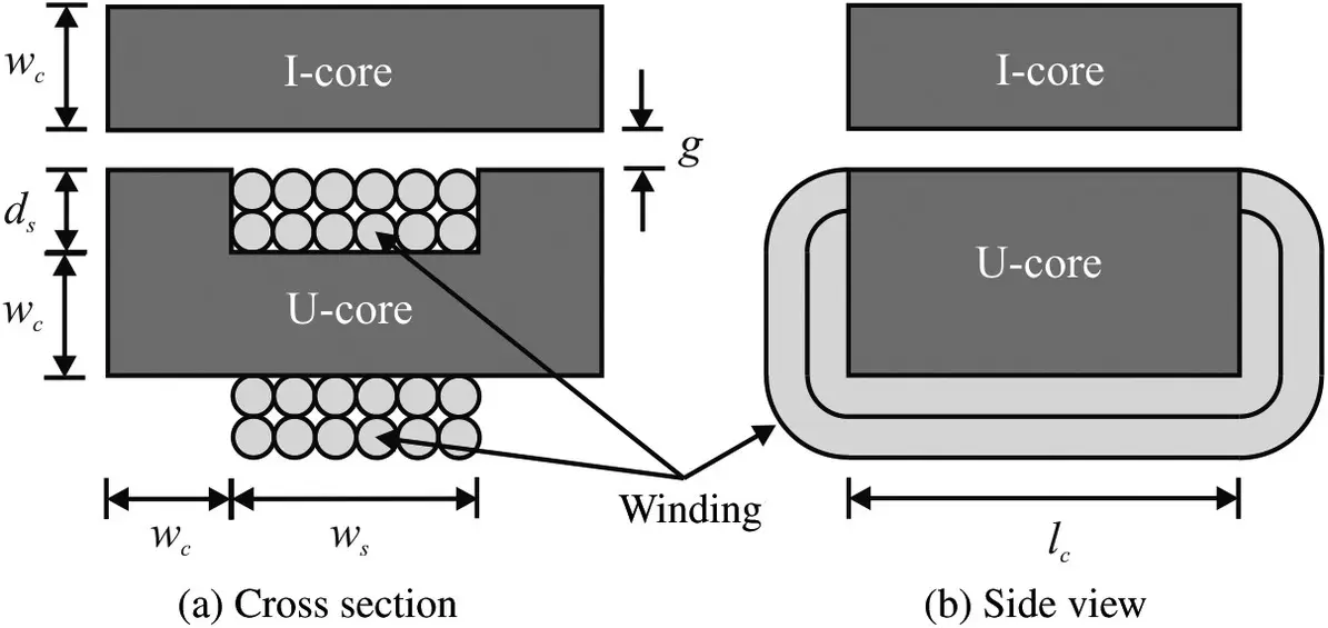
Figure 1.22 UI‐core inductor.
The free parameters in our design are the number of turns N , the slot depth d s, the slot width w s, the core thickness w c, the core depth l c, and the air gap g . Thus, our parameter vector may be expressed as
(1.10-1) 
In (1.10-1), N *is the desired number of turns rather than the actual number of turns N because, as a design parameter, we will let the number of turns be represented as a real number rather than an integer. This is because for large N this variable acts in a more continuous rather than discrete fashion. The actual number of turns is calculated from the desired number as
(1.10-2) 
In order to perform the optimization, we will need to analyze the device. It is assumed that windings occupy the entire slot, that the core is infinitely permeable, and that the fringing and leakage flux components are negligible. Again, for the reader unfamiliar with these terms, the analysis can be taken as a set of arbitrary mathematical equations; we will spend the rest of the book defining and developing more accurate expressions for these quantities.
With these assumptions, the mass of the design may be expressed as
(1.10-3) 
In (1.10-3), ρ mcand ρ wcdenote the mass density of the magnetic core and wire conductor, respectively, and k pfis the fraction of the U‐core window occupied by conductor. Ideally, it would be 1, but 0.7 is a very high number in practice.
The next step is the computation of loss. The power dissipation of the winding at rated current may be expressed as
(1.10-4) 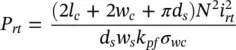
In (1.10-4), σ wcdenotes the conductivity of the wire conductor.
There are constraints both on the inductance, flux density at rated current, and current density at rated current. These quantities may be expressed as
(1.10-5) 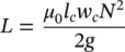
(1.10-6) 
(1.10-7) 
In (10.1‐5)and (1.10-6), μ 0is the magnetic permeability of free space, a constant equal to 4 π 10 −7H/m.
In order to formulate a fitness function, expressions (1.10-1)– (1.10-7)can be sequentially evaluated. Then constraint functions can be evaluated as
(1.10-8) 
(1.10-9) 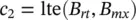
(1.10-10) 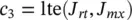
(1.10-11) 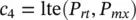
(1.10-12) 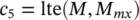
Keeping with (1.9-4), we find the aggregate constraint
(1.10-13) 
We will consider both single‐ and multi‐objective optimization. For the single‐objective case, we will minimize mass and our fitness is given by
(1.10-14) 
For the multi‐objective case, the fitness function will be taken as
(1.10-15) 
In (1.10-14)and (1.10-15), we will take ε = 10 −10.
For our design, let us consider a ferrite material for the core with B mx= 0.617 T and ρ mc= 4680 kg/m 3, and consider copper for the wire with ρ wc= 8890 kg/m 3and J mx= 7.5 A/mm 2. We will take rated current to be 10 A and take the minimum inductance L mnto be 1 mH. Finally, let us take the maximum allowed mass as M mx= 1kg, and the maximum allowed loss to be P mx= 1W.
Table 1.7 Domain of Design Parameters
| Parameter | N | d s(m) | w s(m) | w c(m) | l c(m) | g (m) |
|---|---|---|---|---|---|---|
| Min. value | 1 | 10 −3 | 10 −3 | 10 −3 | 10 −3 | 10 −5 |
| Max. value | 10 3 | 10 −1 | 10 −1 | 10 −1 | 10 −1 | 10 −2 |
| Encoding | log | log | log | log | log | log |
| Chromosome | 1 | 1 | 1 | 1 | 1 | 1 |
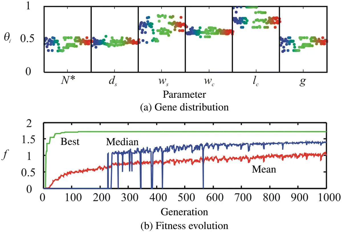
Figure 1.23 Single‐objective optimization study.
Читать дальшеИнтервал:
Закладка:
Похожие книги на «Power Magnetic Devices»
Представляем Вашему вниманию похожие книги на «Power Magnetic Devices» списком для выбора. Мы отобрали схожую по названию и смыслу литературу в надежде предоставить читателям больше вариантов отыскать новые, интересные, ещё непрочитанные произведения.


Обсуждение, отзывы о книге «Power Magnetic Devices» и просто собственные мнения читателей. Оставьте ваши комментарии, напишите, что Вы думаете о произведении, его смысле или главных героях. Укажите что конкретно понравилось, а что нет, и почему Вы так считаете.