Distributed Acoustic Sensing in Geophysics

(1.27)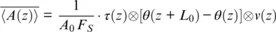

where θ ( z ) is the Heaviside step function, whose value is zero for a negative argument. As expected, the DAS signal is represented ( Equation 1.5) as a convolution of a point spread function with v ( z ).

Spatially integrated signal ( Equation 1.27) was modeled for 10 m gauge length and 50 ns pulsewidth, as shown in Figure 1.5(right panel). The results of modeling ( Equation 1.25) are presented in Figure 1.11(left panel), and the result is converted to geophone‐style data ( Equation 1.26) in the right panel. From a practical point of view, low temporal frequencies, out of the range of interest, can be filtered out, and also spatial antialiasing filtering can be used. It is worth mentioning that the right panel of Figure 1.11demonstrates the real change in polarity of the reflected seismic pulse. Also, spatial integration ( Equation 1.26) acts as statistical averaging, which eliminates the randomness of the “staircasing” in Figure 1.5left panel.

The most valuable geophysical information is delivered by sound waves with frequencies below F MAX= 150 Hz , as higher frequencies are attenuated by the ground. For a speed of sound C = 3000 m / s , this corresponds to an acoustic wavelength C / F MAX= 20 m , so Nyquist’s limit dictates that L G≤ C /2 F MAX= 10 m is the maximum spacing of conventional sensors. Formally, the linear spline approximation G ( z ) of conventional antenna velocity v ( z ) output can be represented using expressions from (Unser, 1999), as:

(1.28)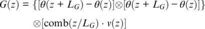

The spatial spectral response of DAS in acoustic angular wavenumber K zcan be represented by Fourier transform ℑ ( K z) following Goodman (2005):

(1.29)

Such spectral responses can be normalized for a constant signal ℑ ( K ) = 1 (see black line in Figure 1.12). The comb function in ( Equation 1.29) is responsible for the repeating of the spatial spectrum with a shift of 2 π /Λ, as is shown by the dotted line. To prevent aliasing, the signal spectrum should be inside Nyquist’s limit, which is shown by the gray vertical line.

Let us compare the conventional velocity sensor with the DAS spectrum, calculated from the spatial resolution expression ( Equation 1.25), by Fourier transform as:

(1.30)

Two cases are presented in Figure 1.12: when the optical pulse length is almost equal to the interferometer gauge length τ = L 0, and when it is half the interferometer gauge length τ = L 0/2 (see dashed and solid blue lines, respectively). The absolute value is presented in the figure to aid comparison between curves. In the second case, we have a gain, which is highlighted by the blue filling. This gain can be explained by signal smearing over a long pulse.

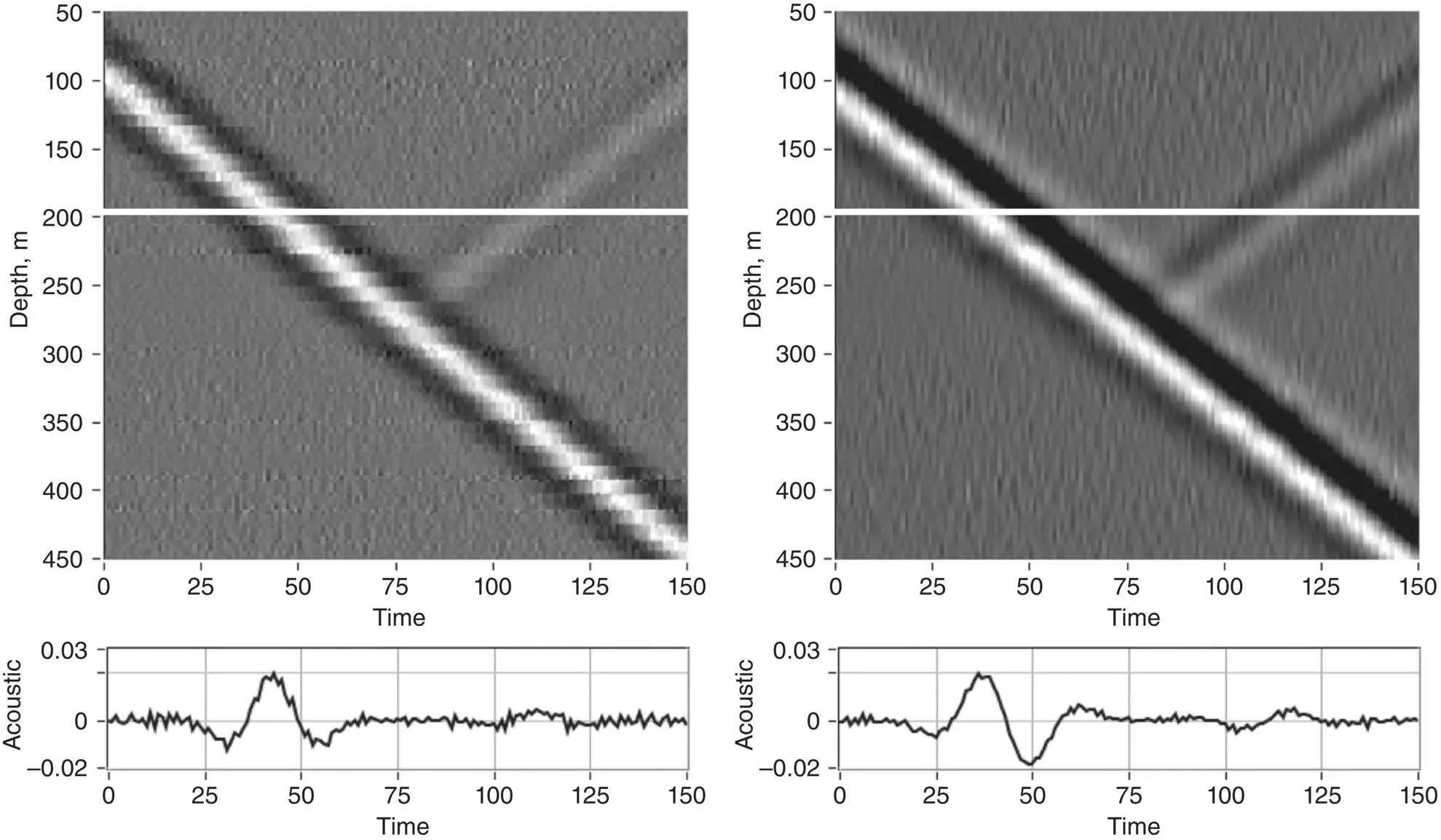
Figure 1.11 Acoustic measurements using DAS: The left panel represents strain rate measurement and the right panel displays ground speed measurement, the transform to which comprises filtering and integration. The signals’ cross‐section along the white line is shown in the bottom panels in radians. The modeled source is shown in the right panel of Figure 1.5.

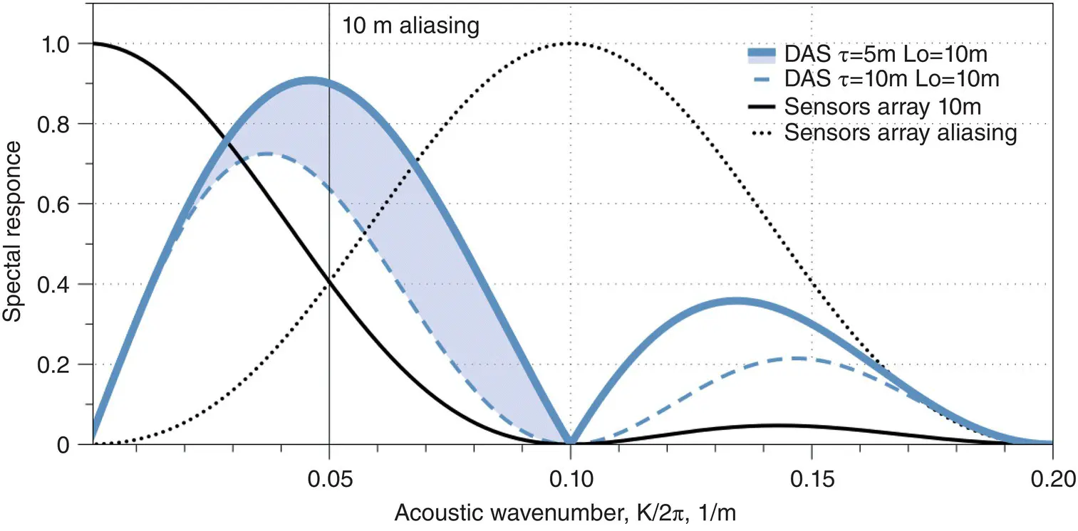
Figure 1.12 Comparison of DAS spectral response with that from a 10 m sensor antenna array.

It seems from Figure 1.12that DAS low frequency sensitivity is significantly lower than that of a geophone. Practically, however, this is not the case, as the geophone noise rises at low frequencies, and this can be characterized by some high‐pass (HP) filters that limit the range to frequencies around 10 Hz (see dotted line in Figure 1.13). However, DAS has the potential to increase the spectral response at low frequencies by increasing interferometer length—for example, from L 0= 10 m to L 0= 30 m (see Figure 1.13). So, potentially, the DAS response can be synthesized from two measurements: with a short interferometer gauge length to deliver high spatial frequency bandwidth, and a long one to deliver low frequency. As the result, full‐frequency coverage can be as good as from a geophone antenna, or possibly even better, as will be shown in a later SNR comparison. An additional advantage over geophones is the large dynamic range of DAS at low frequencies, which will be discussed later.

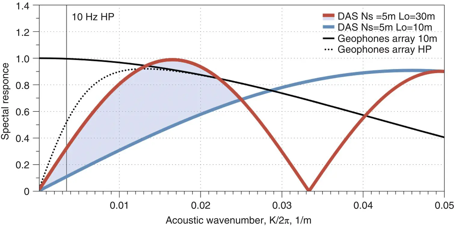
Figure 1.13 Low spatial frequency gain in DAS by using long interferometer.

In the previous section, we analyzed the correspondence between DAS and geophones in the one‐dimensional case and found that “geophone‐style” velocity data can be extracted from DAS signals by spatial integration. However, in 3D analysis, we should consider that DAS is not a velocity sensor but a differential strain sensor. This is a fundamental difference: DAS can measure a component of 3D tensor (strain) but not 3D vector (velocity).

Directionality of the DAS response depends on the fiber optic cable configuration and the cable design, as the device itself is sensitive only to fiber elongation. We will start our consideration where the fiber is placed linearly inside a cable, with no slippage between fiber and cable, nor between the cable and the ground. In this case, fiber displacement will follow ground displacement, and sensitivity will depend on the relative position of fiber and seismic source. A similar mechanical principle was used for the electromagnetic linear strain seismograph to measure variations in the distance between two points of the ground (Benioff, 1935). DAS directional response with respect to incident angle Γ can be found by transformation of the strain tensor components with rotation using geometrical consideration. For a longitudinal (P) apparent wave, it will be cos 2Γ, and for transversal (S) wave sin Γ cos Γ, similar to Benioff (1935) (see Figure 1.14). Detailed analysis and diagrams for Rayleigh and Love waves can be found in Martin et al. (2018).

In vertical seismic profiling (VSP), in the vertical part of the well, both cable and seismic waves are in the same direction for near‐offsets, so the DAS is more sensitive to P‐waves, in which the acoustic displacement vector coincides with the fiber direction. In other applications, such as fracking, the microseismic source is usually on a side of the cable, so shear waves can be effectively detected.