Distributed Acoustic Sensing in Geophysics

From a quantum point of view, we need, for successive phase measurements, a number of interfering photon pairs scattered from points separated by the gauge length distance. In some “bad” points, there are no such pairs, as one point of scattering is faded. A natural way to handle this problem is to reject “bad” unpaired photons by controlling the visibility of the interference pattern. As a result, the shot noise can increase slightly as the price for the dramatic reduction of flicker noise. The rejection of fading points can be practically implemented by assigning a weighting factor to each measurement result and performing a weighted averaging.

This averaging can be done over wavelength if a multi‐wavelength source is used. Alternatively, we can slightly sacrifice spatial resolution and solve the problem by denoising using weighted spatial averaging (Farhadiroushan et al., 2010). The maximum SNR is realized when the weighting factor of each channel is chosen to be inversely proportional to the mean square noise in that channel (Brennan, 1959), meaning the squared interference visibility, V 2, can be used for the weighting factor as:

(1.21)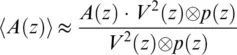

The averaging function p ( z ) = 5 m should optimally be chosen to be compatible with the pulsewidth τ ( z ) = 50 ns , which should be around half the interferometer length L 0= 10 m . With this width of the averaging function, it has no significant effect on the spatial resolution of the DAS. Modeling with and without weighted averaging is presented in Figure 1.9, which demonstrates that significant noise reduction can be achieved. It should be noted that this noise reduction is particularly marked in comparison with the coherent OTDR response, by contrasting with Figure 1.5. Nevertheless, weighted averaging suppresses rather than completely removes the effect of flicker noise, and some channels still demonstrate excessive noise (in addition to shot noise). Hence, the response over all depths at a given time for Figure 1.9will contain spikes for faded channels.

As is explored in Section 1.3, the problem of flicker noise can be overcome by introducing engineered bright scatter zones along the fiber with constant spatial separation and uniform amplitude. Such scatter zones also reflect more photons, and so improve the shot noise detection limitation. In addition, the use of such engineered fiber allows the use of phase‐detection algorithms with improved sensitivity and extended dynamic range.

Figure 1.9 The left‐hand panel shows modeling of raw DAS acoustic data ( Equation 1.12); the right‐hand panel shows the same shot with weighted averaging denoising ( Equation 1.13) applied. The signals’ cross‐section along the white line is shown in the bottom panels in radians. The modeled

source is shown in the right panel of Figure 1.5.

A DAS interrogator measures, in accordance with Equation 1.13, the speed difference between two sections of fiber that are separated by interferometer length L 0(referred to also as the gauge length ), as presented in Figure 1.10. In pulse‐to‐pulse consideration, the DAS response is linearly proportional to the fiber elongation averaged over the gauge length in the nanometer scale, or strain rate in the nanostrain per second scale. The consideration can also be extended to multiple pulses by time integration of the DAS signal. So, if fiber rests initially and ground displacement equals to zero u ( z , t 1) = 0, then:

(1.22)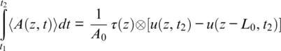

meaning a time integrated DAS signal can be considered as an output of a huge caliper that is measuring fiber elongation between two points with sub‐nanometer precision. This measuring principle is different from that of a geophone but is similar to an electromagnetic linear strain seismograph that can measure changes in distance between two points on the ground (Benioff, 1935).

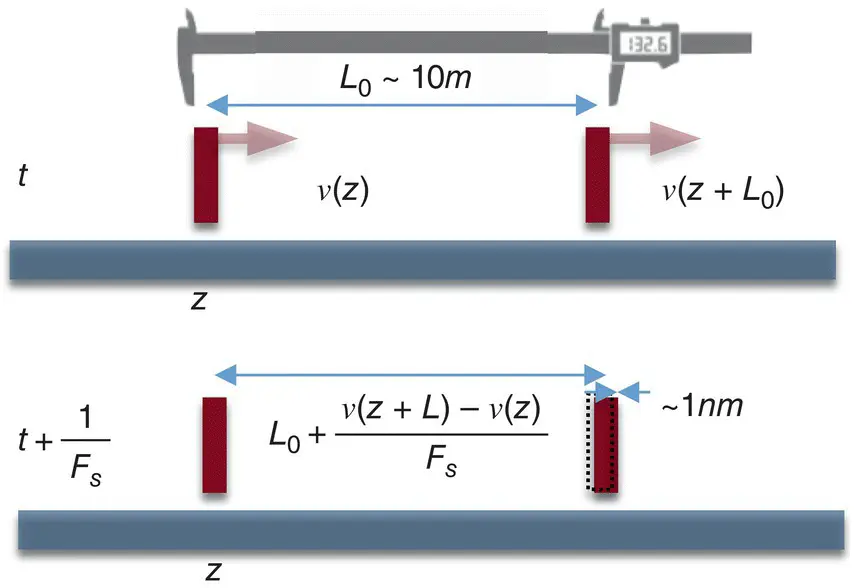
Figure 1.10 Illustration of two time‐consecutive measurements when DAS output is proportional to fiber elongation between two probe pulses.

In this section, we consider how DAS parameters (such as spatial resolution), gauge length, frequency response, and SNR enable DAS to become an effective tool for seismic measurements. Field data are also presented, with DAS output compared to geophone data.

Distributed fiber sensors measure physical parameters of an external environment continuously through the integration properties of light traveling along a lengthy optical path. This is quite different from point sensors, such as geophones, which make an inertial measurement of ground speed at fixed positions (SEAFOM, 2018). The DAS records a local strain rate, which can be converted into particle velocity to allow direct comparison with geophone data. Following Jousset et al. (2018), we can approximately represent DAS signal A ( z , t ) via ground displacement u ( z , t ), where F Sis the DAS sampling frequency and L 0is the gauge length.

(1.23)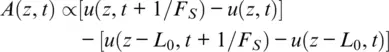

If F S→ ∞, L 0→ 0, then the DAS signal can be presented in a double differential form:

(1.24)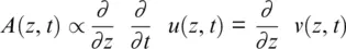

These simplified expressions ( Equations 1.23– 1.24) give us a qualitative sense of the DAS algorithm output. For a subsequent quantitative analysis, we shall need the detailed expression that was obtained in the previous section. Namely, for a nonzero interferometer gauge length L 0and optical pulsewidth τ , averaged over random scattering DAS output, A ( z ) can be represented by Equation 1.15in expanded form:

(1.25)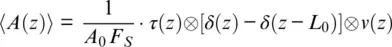

where F Sis sampling frequency and A 0= 115 nm is a scale constant ( Equation 1.14). So, the velocity field can be recovered by spatial integration starting from a motionless point as:

(1.26)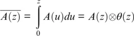

Then DAS signal ( Equation 1.25) can be transformed using shift invariant a ( z 1) ⊗ b ( z 1+ z 2) = a ( z 1+ z 2) ⊗ b ( z 1) to: