Distributed Acoustic Sensing in Geophysics

(1.7)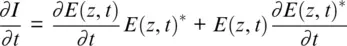

Then using convolution properties ∂ [ a ⊗ b ( t )]/ ∂t = a ⊗ ∂b ( t )/ ∂t , we can find intensity variation via phase shift Φ of backscattered light where there is argument of backscattering complex function:

(1.8)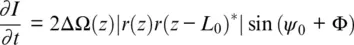

(1.9)

The COTDR signal can be deduced from Equation 1.8if we set L 0= 0 and ψ 0= 0. Even such a simple setup can deliver information on the Doppler shift and hence the ground speed v ( z ) through the intensity variation ∂I / ∂t ∝ Δ v in accordance with Equations 1.3, 1.8. Unfortunately, the proportionality factor contains an oscillation term, so we cannot distinguish positive speed from negative.

The result of computer modeling of a COTDR response on a differential Ricker wavelet for ground speed (Hartog, 2017) is presented in Figure 1.5. The right side shows 1D seismic wave moving in the z direction (in m) with a reflection from an interface with a positive reflection coefficient. Below the image is a time series of apparent velocity, when units are normalized to the expected optical phase shift in radians between points separated by gauge length 10 m. The left side of the figure corresponds to the relative pulse‐to‐pulse variation of the COTDR signal calculated in accordance with Equations 1.8– 1.9. The sign of response changes randomly in accordance with an optical pulsewidth of 50 ns or 5 m. As a result, the signal cannot be effectively accumulated for multiple seismic pulselosityes because of the temperature drift between seismic shots. Temperature drift changes the phase constant of the fiber β 0and, in accordance with Equation 1.4, the effective reflection coefficient r ( z ) also changes. As a result of such drift, every seismic shot will have a unique, random, alternating, speckle‐like signature that cancels the averaging sum. Fortunately, this problem can be overcome by optical phase recovery, when, after similar averaging, average values appear. Thus, the actual DAS output will be a combination of fiber speed information and the unaveraged portion of the random COTDR signal.

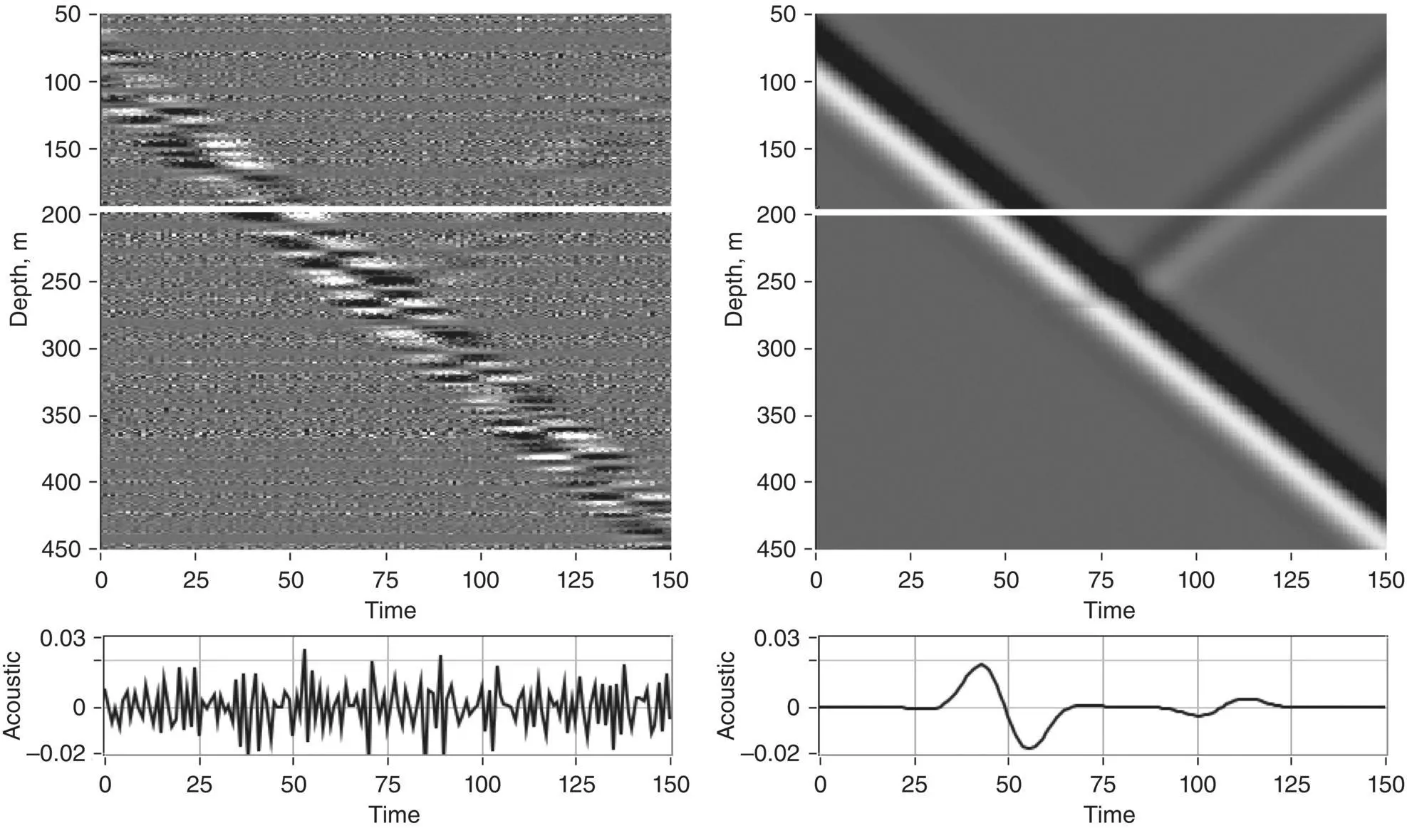
Figure 1.5 COTDR response ( Equation 1.6) shown in the left panel of the simulated signal of a ground velocity wavelet shown in the right panel. The signals’ cross‐section along the white line is shown in the bottom panels in radians.

Source: Based on Correa et al. (2017).

The randomness of the COTDR signal can be reduced through proper control of the external interferometer phase shift ψ 0, which can be achieved in many ways. All these methods are based on the fact that COTDR intensity is random in distance but will vary harmonically depending on the phase, as follows from Equation 1.1(see Figure 1.6). So, phase control can reveal phase information regardless of the random nature of the signal.

We will start our phase analysis with a simple, although not very practical, approach, where the phase shift ψ 0is locked onto a fringe sin( ψ 0+ Φ) ≡ 1. Such an approach was used earlier to analyze the spatial resolution in phase microscopy (Rea et al., 1996). Then Equations 1.8and 1.9can be averaged over an ensemble of delta correlated backscattering coefficients 〈 r ( u ) r ( w )〉 = ρ 2 δ ( u − w ) as:

(1.10)

(1.11)

Equation 1.10demonstrates that the sign of Doppler shift can be measured by DAS with proper phase control. The same data can be extracted directly from phase information, as is clear from Equation 1.11.

So far, we have analyzed the short pulse case, where the pulsewidth is significantly smaller than the external interferometer delay. In reality, such pulses cannot deliver significant optical power, which is necessary for precise measurements. Fortunately, Equations 1.10– 1.11can be generalized for a nonzero length optical pulse e ( z ) directly from Equation 1.5in the same way that an optical incoherent image was obtained in Goodman (2005) using correlation averaging 〈( a ⊗ r 1)( a ⊗ r 2)〉 = 〈 a 2〉 ⊗ 〈 r 1 r 2〉. This expression is valid for an uncorrelated field, generated by random reflection points 〈 r 1( z 1) r 2( z 2)〉 = δ ( z 1− z 2). This calculation confirms that Equation 1.11remains the same, as it represents averaging over different harmonic signals, but Equation 1.10will be reshaped to:

(1.12)

Equation 1.11gives us the possibility to introduce a dimensionless signal as a phase change over a repetition or sampling frequency F Speriod A ( z ) = F S· ∂Φ/ ∂t , and so the DAS output A ( z ) can be represented for pulsewidth τ ( z ) = e ( z ) 2from Equations 1.3, 1.10, and 1.11as:

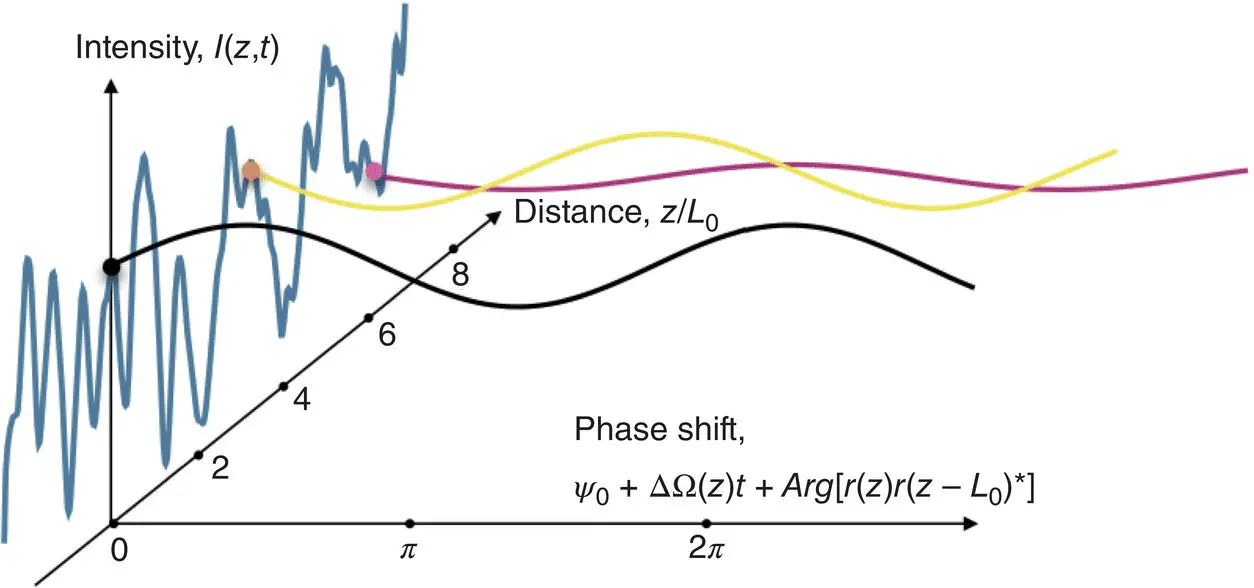
Figure 1.6 Intensity changes are irregular along distance but harmonic along phase shift axis.

(1.13)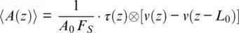

(1.14)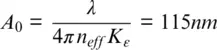

In Equation 1.14, the elongation corresponding to ΔΦ = 1 rad is A 0= 115 nm , calculated for λ = 1550, n eff= 1.468 and K ε= 0.73, which has been measured for conventional fiber (Kreger et al., 2006). The DAS signal is a convolution of pulse shape (as is typical for OTDR‐type distributed sensors) with a measured field, which is the spatial difference in fiber elongation speed of points separated by a gauge length.

Phase measurements can be made in a more practical way than locking the interferometer onto a fringe by using intensity trace I j( z , t ) j = 1, 2, .. P from P multiple interferometers with different phase shifts. Such data can be collected consequentially in P optical pulses, but it reduces sensor bandwidth by P times. Alternatively, the information can be collected for one pulse using a multi‐output optical component, such as a 3×3 coupler. In the general case, the phase shift Φ( z , t ) can be represented (Todd, 2011) via the arctangent function ATAN of the ratio of imaginary Im Z to real part Re Z of linear combinations of intensities: