Distributed Acoustic Sensing in Geophysics

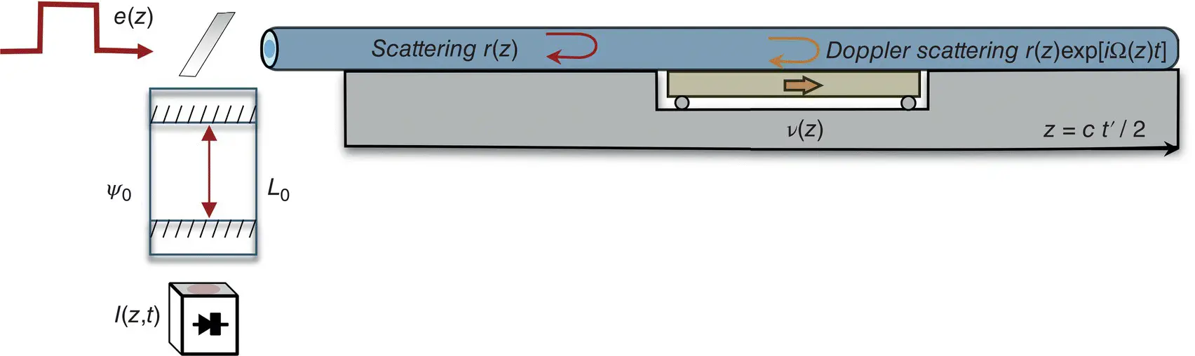
Figure 1.4 DAS optical setup. Distance is proportional to flytime.

Other solutions, such as that shown in Figure 1.3b, contain an embedded delay line that defines the spatial resolution. We will focus our analysis on this class of systems. Another configuration uses optical heterodyne, as shown in Figure 1.3c, where the backscatter signal is continuously mixed with a slightly frequency shifted local oscillator laser. In this case, the elongation along the fiber is measured by computing the difference of the accumulated optical phase between two sections of fiber, and the measurement is carried out at differential frequency f 1− f 2. Although this technique offers a flexible spatial resolution, it requires a laser source with extremely high coherence to achieve reasonable signal‐to‐noise ratio (SNR) performance over several tens of kilometers of fiber. The details of the heterodyne concept are thoroughly covered elsewhere (Hartog, 2017). Another method involves sending multiple pulses of different frequencies, either in series or from pulse to pulse, and then computing the phase of the backscatter signal, as indicated in Figure 1.3d. The phase calculation in this case is similar to first case ( Figure 1.3a).

The theoretical concept of DAS is based on the assumption that the Rayleigh centers have no microscopic motion, but they are “frozen” inside glass during manufacture. In this case, the positions of the centers depend on the macroscopic motion of fiber and can coincide with the ground speed around a buried fiber ( v ). There are two time scales of relevance to DAS: (1) as optical pulse travels with speed c , significantly faster than ground motion, this dictates the spatial resolution; (2) seismic motion is responsible for interference changes pulse to pulse, which can be used to recover the seismic signal. All parameters for both fast and slow motions are summarized in the table of variables at the end of the chapter.

Let us calculate how the intensity of backscattered light changes when a section of fiber is moving with speed v ( z ) under a seismic wave ( Figure 1.4). The Rayleigh centers will move with the fiber, so the frequency of the backscattered light will experience a Doppler shift Ω( z ) proportional to its speed, like for Brillouin scattering (Hartog, 2017). The aim of DAS can be considered as the measurement of Doppler shift for Rayleigh scattering derived from the detected photocurrent. The phase shift can be measured between two separate points in space, and then the resultant Doppler shift can be recovered with spatial integration, as will be shown later in the text. The first step is to analyze changes in intensity between different optical pulses to derive the fiber speed information, which will be equal to the ground speed in a seismic wave.

Consider a coherent optical pulse e ( t ′) that is launched into a single‐mode optical fiber. The backscattered optical field E ( t ′) at time t ′ for light reemerging from the launch end can be expressed as a superimposition of delayed partial fields backscattered with a reflection coefficient r 0( z ) along the fiber axis z (Shatalin et al., 1998). This amplitude coefficient represents coupling between the forward and backward modes. For a speed of light in the fiber c ≈ 2 10 8 m / c , and wave propagation constant β , we can use group and phase delays 2 z / c and , respectively. So, the emerging field will depend on interferometer optical delay, or gauge length, L 0as:

(1.1)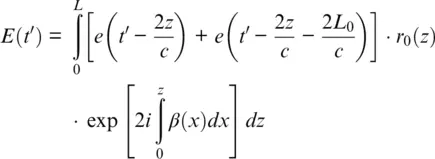

For a regular fiber, the phase shift term in Equation 1.1can be separated into a constant part and a part changing with “slow” time t , representing pulse‐to‐pulse parameter variation with Doppler shift frequency Ω( z ), which is proportional to scattering particle velocity v ( z ) and wavelength frequency ω .

(1.2)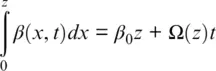

(1.3)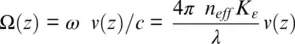

Here the strain coefficient K εrelates the physical and optical length of fiber, n effis fiber effective refractive index, and λ is the laser wavelength. Equations 1.2– 1.3represent a well‐known dualism, when a change in interference can be considered not only as a result of a change in phase, but also as a beating of a frequency due to a Doppler shift. The concept finds application in Doppler lidars, where Rayleigh scattering light contains wind speed information, so the height distribution of the speed can be detected using OTDR (Garnier & Chanin, 1992). The DAS conception is somewhat different: we do not measure the absolute velocity of Rayleigh scatterers, but the difference in such velocity along the gauge length. Another difference is that Rayleigh centers are frozen in a glass of fiber at a melting point of about 800°. Their movement follows the movement of the fiber, and hence very low Doppler frequencies (down to mHz) can be measured.

For simplicity of further calculations, the reflective coefficient r 0( z ) can be redefined as the effective reflective coefficient r ( z ):

(1.4)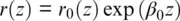

Then, to extract the Doppler shift from the intensity equation, we need to control the phase shift ψ 0between delayed optical fields in the interferometer. So Equation 1.1can be rearranged using Equations 1.2– 1.4to:

(1.5)

Here the convolution symbol ⊗ is used to simplify the expression, and the OTDR scale z = 2 ct ′ for the “fast” time t ′ is used. The convolution commutes with translations (Goodman, 2005), meaning that Equation 1.5can be converted using a ( z 1− z 2) ⊗ b ( z 1) = a ( z 1) ⊗ b ( z 1− z 2) to:

(1.6)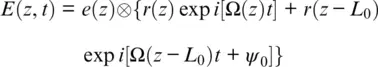

Let us consider first the simple case of short pulse e ( z ) = δ ( z ) when δ is the Dirac delta function. Then convolution can be removed from Equation 1.5because δ ( z ) ⊗ a ( z ) = a ( z ), and the distance variation of Doppler shift ΔΩ( z ) = Ω( z ) − Ω( z − L 0) can be represented via variation of intensity I ( z , t ) = E ( z , t ) E ( z , t )*. The expression in braces in Equation 1.6represents a two‐beam interference, so the intensity will vary harmonically depending on the phase. As we are interested in the intensity change, only the interference term needs be taken into consideration, which can be reshaped using the intensity derivative: