Distributed Acoustic Sensing in Geophysics

(1.15)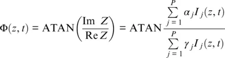

(1.16)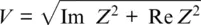

where V is the visibility given by the ratio of peak‐to‐peak intensity variation to average intensity of the interference signal. In particular, for a symmetrical 3×3 coupler, 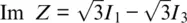and Re Z = I 1− 2 I 2+ I 3. An additional modification of Equation 1.15including phase unwrapping will be discussed in the next section. It is interesting to mention that a heterodyne approach (Hartog et al., 2013) can also use quadrature measurements similar to Equation 1.15, but in that case phase diversity is realized in the OTDR time/distance scale, which can affect spatial resolution. Also, we can mention that the interferometer approach does not need a highly coherent laser, as the optical lengths of interfering rays are nearly compensated (Posey et al., 2000).

The theoretical expression for DAS resolution ( Equation 1.13) was obtained from analysis of an interferometer locked onto a fringe, and it is necessary to test how this is applicable to practical phase measurement algorithms. Also, Equation 1.13contains averaging over a statistical ensemble, and it is important to understand what it means in a real application. To answer the questions, we have compared theoretical values with a simulation based on a 3×3 coupler setup for 100 different random Rayleigh scattering patterns for a wide variety of parameters and found good comparison after averaging. To illustrate this analysis, three optical pulsewidth settings were used for interferometer delay (gauge length) of L 0= 10 m and a ground velocity zone of 40 m ( Figure 1.7a–c).

All traces ( Figure 1.7a–c) correspond to strain measurements rather than to ground velocity profile measurements. If the pulsewidth is small, τ = 10 ns , then averaging is not important, and the correspondence between different phase recovery algorithms are clear ( Figure 1.7a). For a reasonable pulsewidth, τ = 50 ns , only averaged simulation results correspond to theory ( Figure 1.7b). If pulsewidth τ = 100 ns becomes equal to L 0= 10 m in the OTDR scale, then averaging is critical, but after it 100 times averaging correspondence is good ( Figure 1.7c). It is important to mention that this simulation did not include photodetector noise, and noise‐like performance in Figure 1.7c can be explained by the COTDR signal, which will be overlaid on the DAS signal with nonzero pulsewidth. This is a natural limit for increasing SNR by extending pulsewidth; we have a compromise between SNR and signal quality at around L 0= 2 τ . Finally, we can expect that the theoretical expression ( Equation 1.13) can be used for spatial resolution analysis for different phase recovery algorithms after a proper averaging.

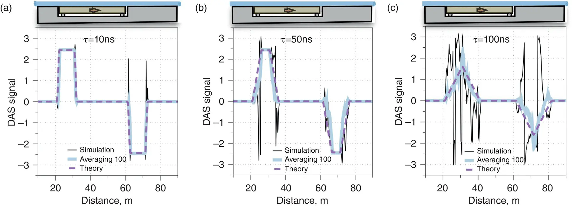
Figure 1.7 Comparison of DAS theoretical response ( Equation 1.13) with simulation for a 3 × 3 coupler.

An acoustic algorithm ( Equation 1.15) transforms the DAS intensity signal into a phase shift proportional to fiber elongation value; a question then is how large can this phase shift be? An algorithm based on such ambiguous function as ATAN( x ) can give a result only inside a limited region. The classic approach to recover large phase changes is unwrapping: stitching together two consecutive points t and t + Δ t from different branches of signal (Itoh, 1982):

(1.17)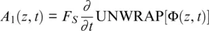

This unwrapping, or phase tracking, concept works only if the phase difference is inside two quadrants:

(1.18)

Equation 1.17makes it possible to measure significant fiber elongation, much longer than the wavelength. If the sampling rate F S= 1/Δ t is higher than the acoustic frequency F , a larger acoustic amplitude can be integrated A 0 F S/2 F ≈ 68 μ over time for F = 50 Hz and F S= 50 kHz . Moreover, even this value has improved, and Equation 1.18gives an idea of this. If the phase is a smooth function, we can differentiate in time Φ( t ) before unwrapping. Then, the first differential linear term is removed, and condition becomes more relaxed:

(1.19)

So, the second order tracking algorithm can be obtained by differentiating the signal before unwrapping:

(1.20)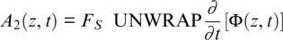

Equation 1.20has an analog in classical optics, where, instead of the wavefront phase gradient, the wrapped curvature of the wavefront can be unwrapped to increase the dynamic range (Servin et al., 2017). A comparison of these algorithms is presented in Figure 1.8using modeling for a harmonic signal with a linearly increasing amplitude. It is visible that both algorithms can recover a significant phase range, but the second order tracking algorithm can deliver in excess of a 10 times larger dynamic range.

Theoretically, even higher order algorithms can be designed by repeating this process using higher order derivatives, but they are noisier as more points are involved in the calculation—as can be seen by comparing Equations 1.18and 1.19. From a practical point of view, the proposed 1D (in time) unwrapping algorithms are error‐free and simple enough to be implemented in real time. Potentially, noise immunity can be improved by transition to 2D (in time and distance) unwrapping, similar to that used in a synthetic aperture radar system (Ghiglia & Pritt, 1998). This solution can extract as much information about the phase as possible, but it is difficult to implement without post‐processing.

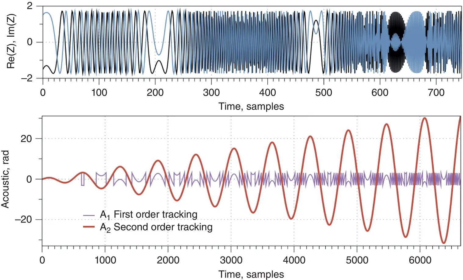
Figure 1.8 Comparison of first and second order tracking algorithms for DAS.

In all phase‐detection schemes, the change in optical phase between the light scattered in two fiber segments is determined, meaning we are measuring the deterministic phase change between two random signals. The randomness of the amplitude of the scattered radiation imposes certain limitations on the accuracy of the sensor, through the introduction of phase flicker noise. The source of flicker noise is an ambiguity: when the fiber is stretched, the scattering coefficient varies, and can become zero. In this case, the differential phase detector generates a noise burst regardless of which optical setup is used. The amplitude of such noise increases with decreasing frequency (as is expected for flicker noise) when the phase difference is integrated into the displacement signal.