Distributed Acoustic Sensing in Geophysics

where comb ( z ) is the Dirac comb function, or sampling operator. If the gauge length is s times larger than sampling distance, L 0= s L S, s = 1, 2…, then r ( z ) = r ( z − L 0), and the reflectivity function r ( z )can be taken out of the brackets:

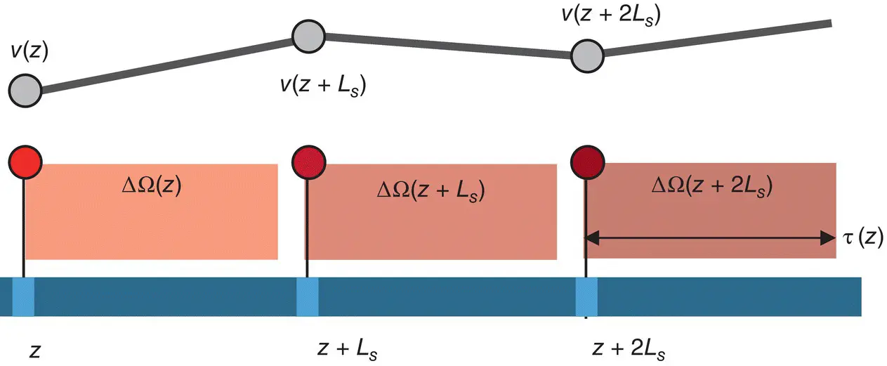
Figure 1.25 Optical fiber with defined scatter center zones and the corresponding Doppler shifted angular frequency sampled between the zones. The length occupied by optical pulse is less than the distance between the zones. The gray line corresponds to spatially integrated DAS output, following a linear spline approximation.

(1.36)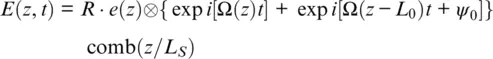

To prevent cross‐interference and fading, the spatial length of the optical pulse should be smaller or equal to the distance between scatter center zones, so the spatial sampling of the optical field ( Equation 1.35) can be represented by a train of pulses:

(1.37)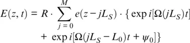

The optical pulses from each zone are separated (see Figure 1.25), so the maximum signal intensity and maximum SNR can be delivered if the pulsewidth is equal to the sampling distance, or τ ( z ) = θ ( z + L S) − θ ( z ), where θ ( z ) is the Heaviside step function whose value is 0 for negative argument and 1 for positive argument. In this case, intensity can be calculated from the interference between pulses with the same index j , and, for each pulse, an acoustic signal A ( z ) = F · ∂Φ/ ∂t , where Φ = ΔΩ( z ) t can be recovered from Equation 1.34using A 0from Equation 1.14as:

(1.38)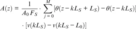

where A 0= 115 nm . Equation 1.38can also be represented in convolution as:

(1.39)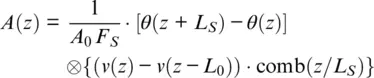

The main parameter for spatial resolution is still the gauge length L 0, and the sampling distance can be chosen to have two points per gauge length L S= L 0/2. We are considering here the physical spatial sampling, which is defined by the optical configuration, keeping in mind that the photocurrent sampling can have a higher rate. The difference from conventional fiber is an absence of averaging, as the detected signal is deterministic for engineered fiber, and excessive noise from non‐averaged components will hence disappear. Also, the generated optical field can be significantly larger than with conventional Rayleigh backscattering, so the shot noise limitation can be reduced significantly.

The velocity field can be recovered by spatial integration starting from a motionless point as:

(1.40)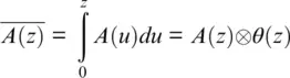

So Equation 1.39can be transformed to:

(1.41)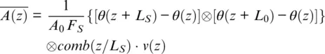

Formally, the engineered fiber DAS signal expression ( Equation 1.41) looks similar to that for standard fiber signal ( Equation 1.27). If, say, L 0= L S, then, in Equation 1.41, the curly expression { } represents a chapeau function for linear spline interpolation (Unser, 1999), In other words, v ( z ) is sampled and linearly interpolated with L Speriod in Equation 1.41without any smearing, as it was for the case of conventional fiber ( Equation 1.27).

The results of modeling ( Equation 1.39) are presented in Figure 1.26, left panel. The spatially integrated version of this signal ( Equation 1.41) was modeled for L 0= 2 L S, and is shown in Figure 1.26, right panel. Low temporal frequencies out of the range of interest can be filtered out, and also spatial antialiasing filtering can be used. It is worth mentioning that the right panel of Figure 1.26is very similar to the original pulse ( Figure 1.5), which demonstrates the real change of polarity of the reflected seismic pulse. Compared with Figure 1.10(conventional fiber), Figure 1.26shows better SNR and signal amplitude stability than with conventional fiber, and a more uniform size of the step in the “staircase” in the left panel, which can be easily filtered out.

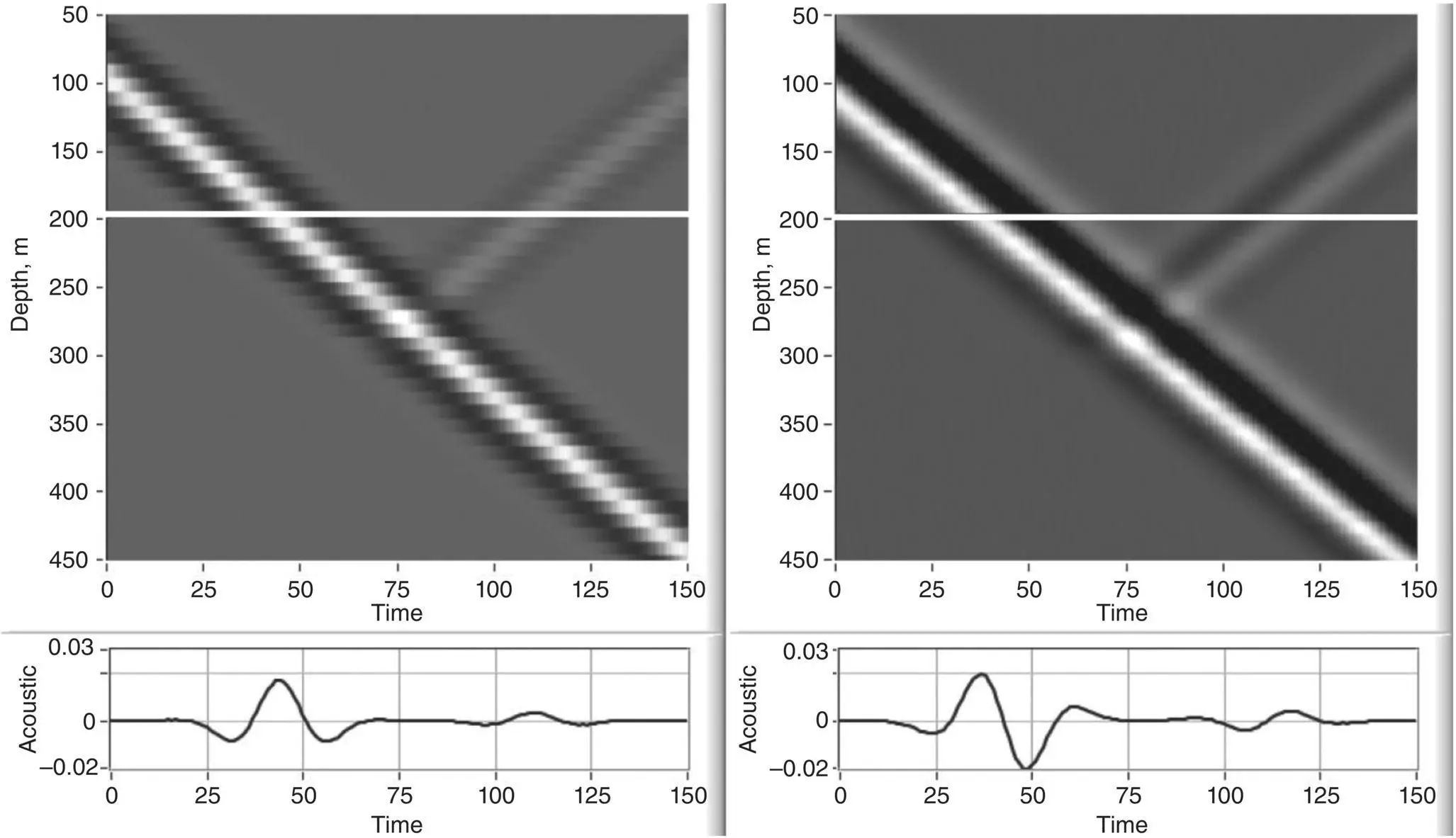
Figure 1.26 Acoustic measurements using DAS with precision engineered fiber: The left panel represents strain rate measurement ( Equation 1.39) and the right panel displays ground speed measurement ( Equation 1.41) after filtering and integration. The signals’ cross‐section along the white line is shown in the bottom panels in radians. The modeled source is shown in the right panel of Figure 1.5.

The spatial spectral response in the wavenumber domain K zcan be represented by Fourier transform ℑ :

(1.42)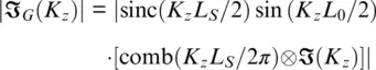

where ℑ ( K z) is the spatial spectral response of the seismic wave. Comparisons of DAS with engineered fiber spectral response for spatial sampling equal to the gauge length and half of gauge length are presented in Figure 1.27based on Equation 1.41. For the high spatial sampling, we have a gain in the frequency range, which is highlighted by the gray filling. Moreover, it is easy to filter out the aliased component for high sampling as the spectral density is zero for maximum frequency, seen by comparing the position of the black and gray vertical lines in Figure 1.27. This advantage can explain the absence of “staircasing” and the smooth output in Figure 1.26right panel. An additional advantage of high sampling is that, for a typical L 0= L G= 5 m , the sampling is twice or even three times smaller than the sensor separation in a geophone array. This spatial frequency margin is useful because DAS timing is different from analog geophones. For a geophone antenna, we can filter out high‐frequency space‐time components in the time domain by electrically filtering individual channels before sampling to prevent spatial aliasing. This approach is ineffective for DAS when the time sampling acts directly on the rapidly changing photocurrent. The problem can be solved for DAS by mechanical filtering in the acoustic area using a special design of the sensing cable, as in Carroll & Huber (1986). An alternative approach involves some oversampling in the spatial domain, and the result is not completely independent. Subsequent filtering then removes high spatial frequencies and prevents aliasing.