Distributed Acoustic Sensing in Geophysics

Finally, we can neglect the comb function in Equation 1.42, following which Equation 1.42is exactly equivalent to the expression for a conventional fiber ( Equation 1.30) with pulsewidth equal to the scattering period L S= τ = 5 m .

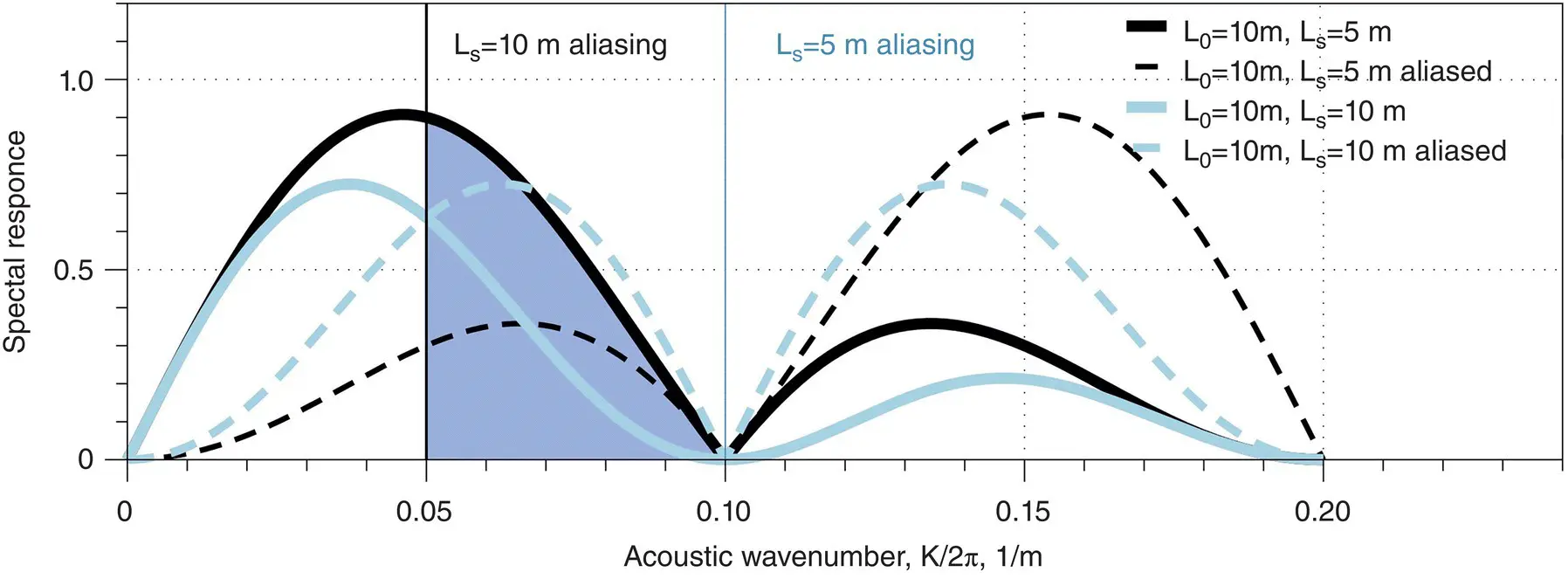
Figure 1.27 Comparison of DAS with engineered fiber spectral response for special sampling equal to gauge length (black) and half of gauge length (gray).

DAS with engineered fiber combines the benefits of a distributed sensor, giving full coverage, with the high sensitivity of point sensors such as geophones. The scatter centers are precisely engineered along the length of the fiber and not distributed randomly as for standard fiber (see Figure 1.28). This allows the backscattered signal to be downsampled precisely and optimum spectral response to be obtained.

The DAS signal with engineered fiber, as expressed in Equation 1.39, can be considered as a staircase function with differential velocity sampling L S: when sampled over each staircase distance L S, the expression in the square brackets will be eliminated from Equation 1.39, and, therefore, the corresponding sinc function in Equation 1.43will also be eliminated. As a result, the DAS signal with engineered fiber will be defined by ( v ( z ) − v ( z − L 0)), or comb filters in the spectral domain:

(1.43)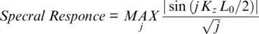

Equation 1.43also includes a gain that can be obtained from synthetic gauge length optimization. With this approach, low spectral frequencies can be measured by adding a few consecutive downsampled signals. From a physical point of view, it means that the combination of multiple gauge lengths L 0can be used to form a single long gauge length. The SNR for the resultant gauge length j L 0will decrease proportionally to in a shot noise limited DAS—see denominator in Equation 1.43. High spatial frequencies can still be measured with original gauge length L 0without any loss of spatial resolution. Potentially, we can maximize the spectral response by choosing a proper averaging factor j for any spectral band, as is expressed in Equation 1.43. A simple practical implementation for optimizing both low and high spatial frequency can be realized by sliding a leaky distance integration of DAS signal similar to how it was done for velocity recovery ( Equation 1.41).

The ultimate spectral response of DAS with standard ( Equation 1.30) and engineered ( Equation 1.43) fiber compared to that from a geophone array is shown in Figure 1.28. The pulsewidth of the DAS is the same as distance between scatter centers in engineered fiber τ = L S= 5 m , and the gauge length is the same as the distance between geophones L G= L 0= 10 m . In summary, downsampling of the DAS signal with engineered fiber can improve the spectral response as compared to standard fiber with the same gauge length. However, DAS with standard fiber can provide a wide spectral response without aliasing, as is shown in Figure 1.28.

DAS sensitivity can be calculated for a fundamental limit—the shot noise generated by the number of photons detected. Let us estimate the photon number N per second based on input peak power P 0= 1 W , which is near to the maximum optical connector power damage threshold (De Rosa, 2002). The backscattered intensity can be found from the typical scattering coefficient for SM fiber R BS= 82 dB for a 1 ns pulse (Ellis, 2007). For an optical pulsewidth τ = 50 ns , the energy quant for λ = 1550 nm is hυ = 1.28 · 10 −19 J . We consider a relatively short fiber length, L = 2000 m , to neglect nonlinear effects (Martins et al., 2013) and suppose that light is collected over an integration length L P= 5 m :

(1.44)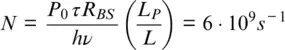

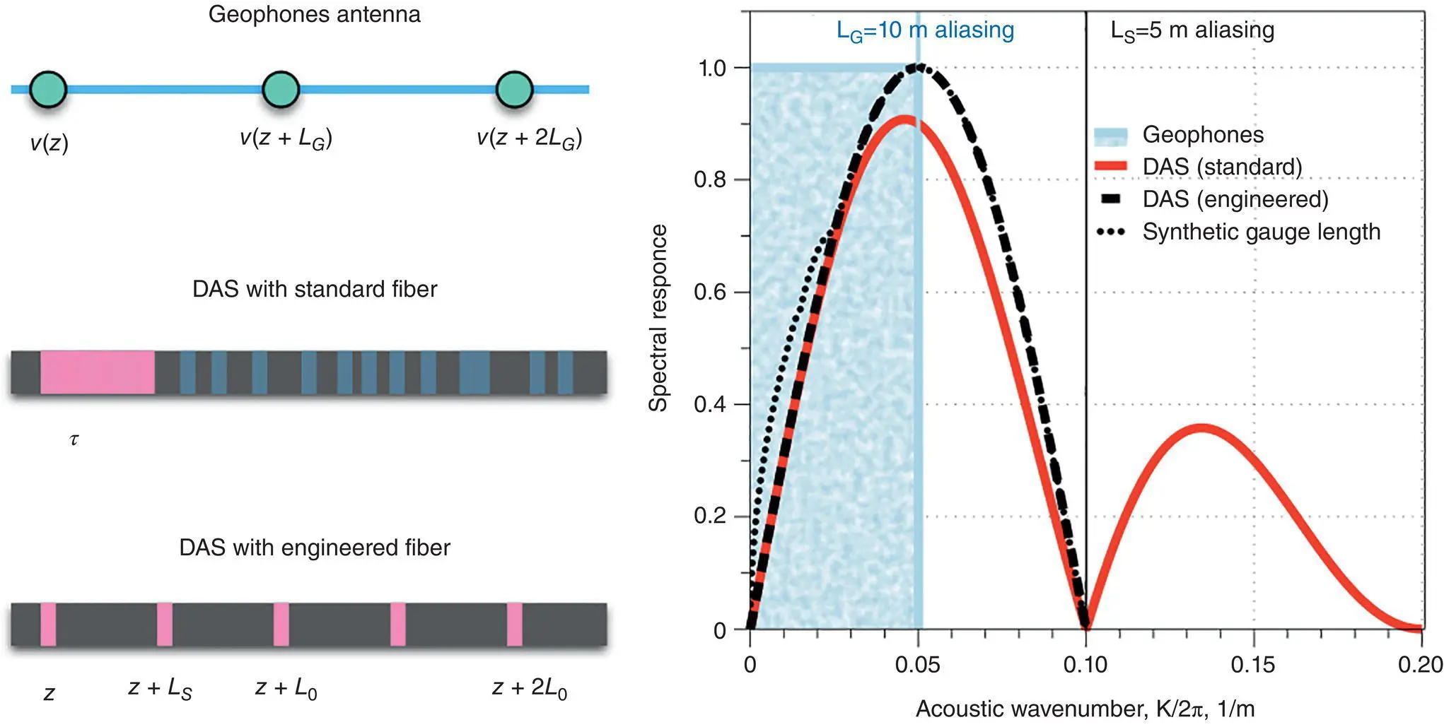
Figure 1.28 Ultimate SNR spectral response of DAS with standard and engineered fiber and geophone antenna. Pulse width of DAS is the same as distance between scatter centers along engineered fiber—5 m, and gauge length of DAS is the same as distance between geophones—10 m.

The shot or Poisson noise limit for phase measurement Φ minis proportional to , where the coefficient depends on the phase‐detection approach. For a classical phase‐locked homodyne, only half of the photons reach the photodetector when the interferometer operates in quadrature, and so the noise is . For both heterodyne and/or homodyne phase detection, the photons number halves again (Kazovsky, 1989), as sine and cosine signal components should be measured independently, and so the noise rises to . Direct photodetection at λ = 1550 nm is not sufficiently sensitive, so DAS usually uses an erbium doped fiber amplifier (EDFA) to boost the signal, which introduces additional noise. This noise can be simply represented by a noise figure N F≈ 3, which can be reached with appropriate optical filtering as explained in Kirkendall & Dandridge (2004). In this case, the shot noise limit is then given by:

(1.45)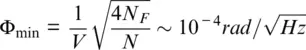

where visibility, V = 0.5, includes all other system imperfections such as polarization mismatch. Equation 1.45represents the white noise level for 1 second time integration of the DAS signal. For engineered fiber, the number of photons can be up to 100 times larger than for conventional Rayleigh backscattering, so the noise will be 10 times smaller.

Another advantage of DAS with engineered fiber is a wider dynamic range that is defined as the ratio of the maximum detectable signal to the noise level. The typical geophone bandwidth is Δ F = 100 Hz , so the minimum strain level ε mindetectable for DAS for gauge length L 0= 10 m within the same detection bandwidth is:

(1.46)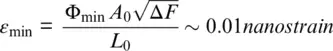

where A 0= 115 nm is the elongation corresponding to one radian phase shift ( Equation 1.14).

Experimental measurements with conventional fiber DAS found a value three times higher, at 0.03 nanostrain (Miller et al., 2016). In this case, there was some extra flicker noise, as discussed earlier (see Figure 1.11). Here, a spiky noise structure corresponds to algorithm discontinuities that amplify photodetector noise, with a spectrum after DAS signal time integration, which is ∝ F −1. The typical low frequency limit when excessive noise starts to dominate over shot noise is between 10 and 100 Hz, depending on the fiber conditions.