Daniel J. Duffy - Numerical Methods in Computational Finance

We state this theorem in more general terms: consistency and stability of a multistep scheme are sufficient for convergence.

Finally, the discussion in this section is also applicable to systems of ODEs. For more discussions, we recommend Henrici (1962) and Lambert (1991).

Finally, we present four finite difference schemes for the IVP (2.31)and their generating polynomials as defined by Equations (2.34):

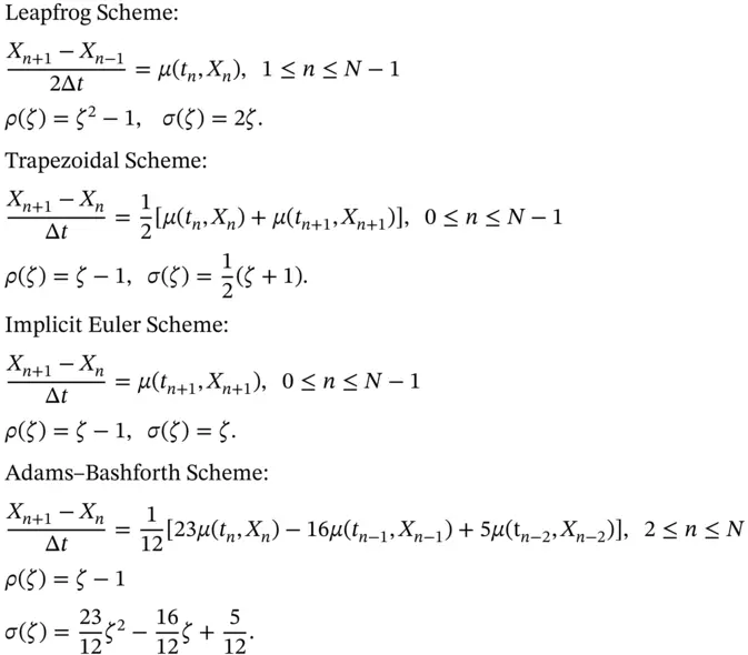
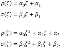
We recommend that you verify the results using the forms of the generating polynomials for one-step and two-step methods, respectively. The general forms are:

We now discuss special classes of ODEs that arise in practice and whose numerical solution demands special attention. These are called stiff systems whose solutions consist of two components; first, the transient solution that decays quickly in time, and second, the steady-state solution that decays slowly. We speak of fast transient and slow transient , respectively. As a first example, let us examine the scalar linear initial value problem:

(2.40)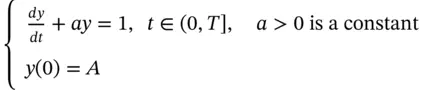

whose exact solution is given by:

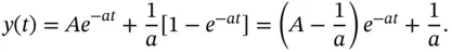
In this case the transient solution is the exponential term, and this decays very fast (especially when the constant a is large) for increasing t . The steady-state solution is a constant, and this is the value of the solution when t is infinity. The transient solution is called the complementary function , and the steady-state solution is called the particular integral (when ), the latter including no arbitrary constant. The stiffness in the above example is caused when the value a is large; in this case traditional finite difference schemes can produce unstable and highly oscillating solutions. One remedy is to define very small time steps. Special finite difference techniques have been developed that remain stable even when the parameter a is large. These are the exponentially fitted schemes , and they have a number of variants. The variant described in Liniger and Willoughby (1970) is motivated by finding a fitting factor for a general initial value problem and is chosen in such a way that it produces an exact solution for a certain model problem. To this end, let us examine the scalar ODE:

(2.41)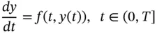

and let us approximate it using the Theta method :

(2.42)

where the parameter has not yet been specified. We determine it using the heuristic that this so-called Theta method should be exact for the linear constant-coefficient model problem :

(2.43)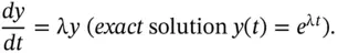

Based on this heuristic and by using the exact solution from (2.43)in scheme (2.42) , we get the value (you should check that this formula is correct; it is a bit of algebra). We get:

(2.44)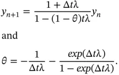

Note: this is a different kind of exponential fitting.

We need to determine if this scheme is stable (in some sense). To answer this question, we introduce some concepts.

Definition 2.3The region of (absolute) stability of a numerical method for an initial value problem is the set of complex values for which all discrete solutions of the model problem (2.43)remain bounded when n approaches infinity.

Definition 2.4A numerical method is said to be A-stable if its region of stability is the left-half plane, that is:

Returning to the exponentially fitted method, we can check that it is A-stable because for all we have , and this condition can be checked using the scheme (2.42)for the model problem (2.43).

We can generalise the exponential fitting technique to linear and non-linear systems of equations. In the case of a linear system, stiffness is caused by an isolated real negative eigenvalue of the matrix A in the equation:

(2.45)

where and A is a constant matrix with eigenvalues and eigenvectors

The solution of Equation (2.45)is given by:

where are arbitrary constants and is a particular integral. In this case we can employ exponential fitting by fitting the dominant eigenvalues which can be computed by the Power method , for example.