Daniel J. Duffy - Numerical Methods in Computational Finance
Здесь есть возможность читать онлайн «Daniel J. Duffy - Numerical Methods in Computational Finance» — ознакомительный отрывок электронной книги совершенно бесплатно, а после прочтения отрывка купить полную версию. В некоторых случаях можно слушать аудио, скачать через торрент в формате fb2 и присутствует краткое содержание. Жанр: unrecognised, на английском языке. Описание произведения, (предисловие) а так же отзывы посетителей доступны на портале библиотеки ЛибКат.

- Название:Numerical Methods in Computational Finance
- Автор:
- Жанр:
- Год:неизвестен
- ISBN:нет данных
- Рейтинг книги:4 / 5. Голосов: 1
-
Избранное:Добавить в избранное
- Отзывы:
-
Ваша оценка:
Numerical Methods in Computational Finance: краткое содержание, описание и аннотация
Предлагаем к чтению аннотацию, описание, краткое содержание или предисловие (зависит от того, что написал сам автор книги «Numerical Methods in Computational Finance»). Если вы не нашли необходимую информацию о книге — напишите в комментариях, мы постараемся отыскать её.
Part A Mathematical Foundation for One-Factor Problems
Chapters 1 to 7 introduce the mathematical and numerical analysis concepts that are needed to understand the finite difference method and its application to computational finance.
Part B Mathematical Foundation for Two-Factor Problems
Chapters 8 to 13 discuss a number of rigorous mathematical techniques relating to elliptic and parabolic partial differential equations in two space variables. In particular, we develop strategies to preprocess and modify a PDE before we approximate it by the finite difference method, thus avoiding ad-hoc and heuristic tricks.
Part C The Foundations of the Finite Difference Method (FDM)
Chapters 14 to 17 introduce the mathematical background to the finite difference method for initial boundary value problems for parabolic PDEs. It encapsulates all the background information to construct stable and accurate finite difference schemes.
Part D Advanced Finite Difference Schemes for Two-Factor Problems
Chapters 18 to 22 introduce a number of modern finite difference methods to approximate the solution of two factor partial differential equations. This is the only book we know of that discusses these methods in any detail.
Part E Test Cases in Computational Finance
Chapters 23 to 26 are concerned with applications based on previous chapters. We discuss finite difference schemes for a wide range of one-factor and two-factor problems.
This book is suitable as an entry-level introduction as well as a detailed treatment of modern methods as used by industry quants and MSc/MFE students in finance. The topics have applications to numerical analysis, science and engineering.
More on computational finance and the author’s online courses, see www.datasim.nl.
Numerical Methods in Computational Finance — читать онлайн ознакомительный отрывок
Ниже представлен текст книги, разбитый по страницам. Система сохранения места последней прочитанной страницы, позволяет с удобством читать онлайн бесплатно книгу «Numerical Methods in Computational Finance», без необходимости каждый раз заново искать на чём Вы остановились. Поставьте закладку, и сможете в любой момент перейти на страницу, на которой закончили чтение.
Интервал:
Закладка:
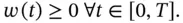
Lemma 2.1 (Positivity).Let the operator  be defined in Equation (2.1), and let
  be a well-behaved function satisfying the inequalities:
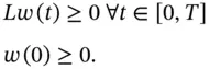
Then the following result holds true:
Roughly speaking, this lemma states that you cannot get a negative solution from positive input.
You can verify it by examining Equation (2.2)because all terms are positive.
The following result gives bounds on the growth of  .
.
Theorem 2.1Let  be the solution of Equation (2.1). Then:
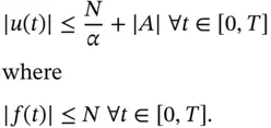
This result states that the value of the solution is bounded by the input data. In other words, it is a well-posed problem .
We wish to replicate these properties in our difference schemes for Equation (2.1).
For completeness, we show the steps to be executed in order to produce the result in Equation (2.2).
(2.3) 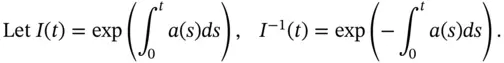
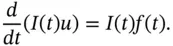
Then from Equation (2.1)we see:
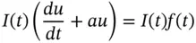
or:
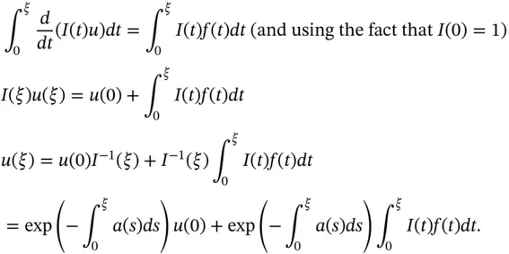
Integrating this equation between  and
and  gives:
This style of mathematical analysis will be used in other contexts in this book, for example when transforming convection-diffusion-reaction equations (in particular, the Black–Scholes equation) to adjoint form .
2.2.2 Rationale and Generalisations
The IVP Equation (2.1)is a model for all the linear time-dependent differential equations that we encounter in this book. We no longer think in terms of scalar problems in which the functions in Equation (2.1)are scalar-valued, but we can view an ODE at different levels of abstraction. To this end, we focus on the generic homogeneous ODE with solution  :
:
(2.4) 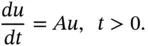
This equation subsumes several special cases:
1 The variable is a square matrix, and then Equation (2.4)represents a system of ODEs. This is a very important area of research having many applications in science, engineering, and finance.
2 The variable is an ordinary or partial differential operator, and then Equation (2.4)represents an ODE in a Hilbert or Banach space.
3 The variable is a tridiagonal or block tridiagonal matrix that originates from a semi-discretisation in space of a time-dependent partial differential equation (PDE) using the Method of Lines (MOL) as discussed in Chapter 20.
4 The formal solution of (2.4)is:(2.5) In other words, we express the solution in terms of the exponential function of a matrix or of a differential operator. In the former case, there are many ways to compute the exponential of a matrix (see Moler and Van Loan (2003)).
5 The solution of Equation (2.4)can be simplified by matrix or operator splitting of the operator : (2.6)For example, we can split a matrix into two simpler matrices, or we can split an operator into its convection and diffusion components. In other words, we solve Equation (2.4)as a sequence of simpler problems in (2.6). These topics will be discussed in Chapters 18, 22, and 23.
6 The initial value problem (2.1)was originally used as a model test of finite difference methods in (Dahlquist (1956)). The resulting results and insights are helpful when dealing more complex IVPs.
Finally, this chapter and Chapter 3are recommended for readers who may not be familiar with ODE theory and ODE numerics. It is a prerequisite before moving to partial differential equations.
2.3 DISCRETISATION OF INITIAL VALUE PROBLEMS: FUNDAMENTALS
We now discuss finding an approximate solution to Equation (2.1)using the finite difference method . We introduce several popular schemes as well as defining standardised notation.
The interval or range where the solution of Equation (2.1)is defined is  . When approximating the solution using finite difference equations, we use a discrete set of points in
  where the discrete solution will be calculated. To this end, we divide
  into
into  equal intervals of length
  , where
  is a positive number called the step size . (We also use the symbol
  to denote the step size in many cases.) We number these discrete points as shown in Figure 2.1. In general all coefficients and discrete functions will be defined at these mesh points only. We adopt the following notation:
(2.7) 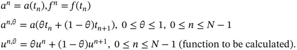
Интервал:
Закладка:
Похожие книги на «Numerical Methods in Computational Finance»
Представляем Вашему вниманию похожие книги на «Numerical Methods in Computational Finance» списком для выбора. Мы отобрали схожую по названию и смыслу литературу в надежде предоставить читателям больше вариантов отыскать новые, интересные, ещё непрочитанные произведения.


Обсуждение, отзывы о книге «Numerical Methods in Computational Finance» и просто собственные мнения читателей. Оставьте ваши комментарии, напишите, что Вы думаете о произведении, его смысле или главных героях. Укажите что конкретно понравилось, а что нет, и почему Вы так считаете.