Computational Statistics in Data Science

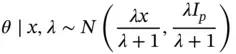
The posterior distribution of (given ) is

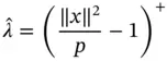
If the true value of is unknown, it is often estimated from the marginal distribution of , via maximum‐likelihood estimation as

Robert and Casella [4] consider estimating 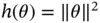using the posterior mean . Under a quadratic loss, the Bayes estimator is

The risk for

is difficult to obtain analytically (although not impossible, see Robert and Casella [4]). Instead, we can estimate the risk over a grid of values using Monte Carlo. To do this, we fix choices over a grid, and for each , generate Monte Carlo samples from yielding estimates

The resulting estimate of the risk is an ‐dimensional vector of means, for which we can utilize the sampling distribution in Theorem 1to construct large‐sample confidence regions. An appropriate choice of a sequential stopping rule here is the relative‐magnitude sequential stopping rule, which stops simulation when the Monte Carlo variance is small relative to the average risk over all values of considered. It is important to note that the risk at a particular could be zero, but it is unlikely.

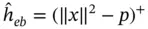
For illustration, we set and simulate a data point from the true model with . To evaluate risk we choose a grid of values with . In order to assess the appropriate Monte Carlo sample size , we set so that at least Monte Carlo samples are obtained. With , and estimated using the sample covariance matrix, the sequential stopping rule terminates simulation at 21 100 steps. Figure 2demonstrates the estimated risk at iterations and the estimated risk at termination. Pointwise Bonferroni corrected confidence intervals are presented as an indication of variability for each component 1 .

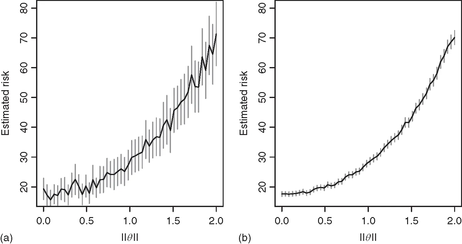
Figure 2 Estimated risk at (a) and at (b) with pointwise Bonferroni corrected confidence intervals.

Consider the biomedical oxygen demand (BOD) data collected by Marske [39] where BOD levels were measured periodically from cultured bottles of stream water. Bates and Watts [40] and Newton and Raftery [41] study a Bayesian nonlinear model with a fixed rate constant and an exponential decay as a function of time. The data is available in Bates and Watts [40], Section A4.1]. Let , be the time points, and let be the BOD at time . Assume for and . Newton and Raftery [41] assume a default prior on , , and a transformation invariant design‐dependent prior for such that , where is an where the th element of . The resulting posterior distribution of is intractable and up to normalization and can be written as