Computational Statistics in Data Science

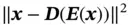
Autoencoder is first introduced in Rumelhart et al . [16] as a model with the main goal of learning a compressed representation of the input in an unsupervised way. We are essentially creating a network that attempts to reconstruct inputs by learning the identity function. To do so, an autoencoder can be divided into two parts, (encoder) and 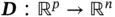(decoder), that minimize the following loss function w.r.t. the input :

The encoder ( ) and decoder ( ) can be any mappings with the required input and output dimensions, but for image analysis, they are usually CNNs. The norm of the distance can be different, and regularization can be incorporated. Therefore, a more general form of the loss function is

(3)

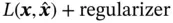
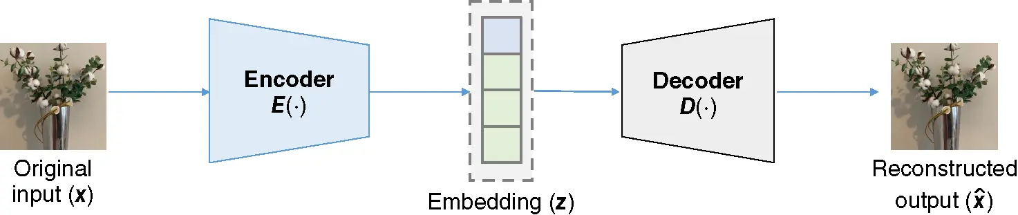
Figure 5 Architecture of an autoencoder.

Source : Krizhevsky [14]

where is the output of an autoencoder, and represents the loss function that captures the distance between an input and its corresponding output.

The output of the encoder part is known as the embedding, which is the compressed representation of input learned by an autoencoder. Autoencoders are useful for dimension reduction, since the dimension of an embedding vector can be set to be much smaller than the dimension of input. The embedding space is called the latent space, the space where the autoencoder manipulates the distances of data. An advantage of the autoencoder is that it can perform unsupervised learning tasks that do not require any label from the input. Therefore, autoencoder is sometimes used in pretraining stage to get a good initial point for downstream tasks.

Many different variants of the autoencoder have been developed in the past years, but the variational autoencoder (VAE) is the one that achieved a major improvement in this field. VAE is one of the frameworks, which attempts to describe an observation in latent space in a probabilistic manner. Instead of using a single value to describe each dimension of the latent space, the encoder part of VAE uses a probability distribution to describe each latent dimension [17].

Figure 6shows the structure of the VAE. The assumption is that each input data is generated by some random process conditioned on an unobserved random latent variable . The random process consists of two steps, where is first generated from some prior distribution , and then is generated from a conditional distribution . The probabilistic decoder part of VAE performs the random generation process. We are interested in the posterior over the latent variable , but it is intractable since the marginal likelihood is intractable. To approximate the true posterior, the posterior distribution over the latent variable is assumed to be a distribution parameterized by .

Given an observed dataset , the marginal log‐likelihood is composed of a sum over the marginal log‐likelihoods of all individual data points: , where each marginal log‐likelihood can be written as

(4)

where the first term is the KL divergence [18] between the approximate and the true posterior, and the second term is called the variational lower bound. Since KL divergence is nonnegative, the variational lower bound is defined as

(5)

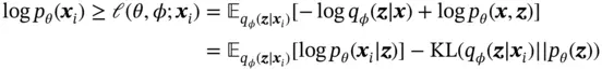
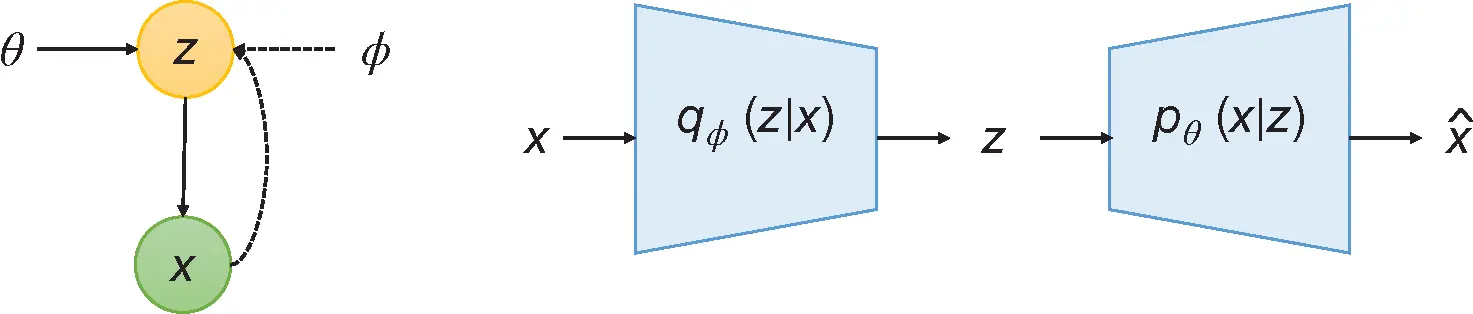
Figure 6 Architecture of variational autoencoder (VAE).

Therefore, the loss function of training a VAE can be simplified as

(6)

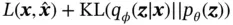
where the first term captures the reconstruction loss, and the second term is regularization on the embedding. To optimize the loss function ( 6), a reparameterization trick is used. For a chosen approximate posterior , the latent variable is approximated by