Computational Statistics in Data Science

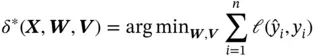
We want to choose the weights and biases in such a way that they minimize the sum of squared errors within a given dataset. Similar to the general supervised learning approach, we want to find an optimal prediction such that

(1)

where 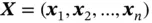, and is cross‐entropy loss.

(2)

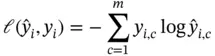
where is the total number of classes; if the th sample belongs to class , otherwise it is equal to 0; and is the predicted score of the th sample belonging to class .

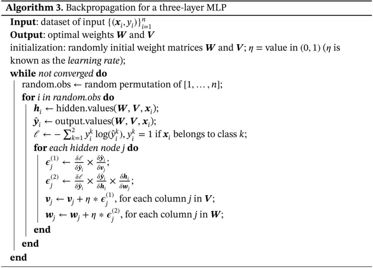
Function ( 1) cannot be minimized through differentiation, so we must use gradient descent. The application of gradient descent to MLPs leads to an algorithm known as backpropagation. Most often, we use stochastic gradient descent as that is far faster. Note that backpropagation can be used to train different types of neural networks, not just MLP.

We would like to address the issue of possibly being trapped in local minima, as backpropagation is a direct application of gradient descent to neural networks, and gradient descent is prone to finding local minima, especially in high‐dimensional spaces. It has been observed in practice that backpropagation actually does not typically get stuck in local minima and generally reaches the global minimum. There do, however, exist pathological data examples in which backpropagation will not converge to the global minimum, so convergence to the global minimum is certainly not an absolute guarantee. It remains a theoretical mystery why backpropagation does in fact generally converge to the global minimum, and under what conditions it will do so. However, some theoretical results have been developed to address this question. In particular, Gori and Tesi [7] established that for linearly separable data, backpropagation will always converge to the global solution.

So far, we have discussed a simple MLP with three layers aimed at classification problems. However, there are many extensions to the simple case. In general, an MLP can have any number of hidden layers. The more hidden layers there are, the more complex the model, and therefore the more difficult it is to train/optimize the weights. The model remains almost exactly the same, except for the insertion of multiple hidden layers between the first hidden layer and the output layer. Values for each node in a given layer are determined in the same way as before, that is, as a nonlinear transformation of the values of the nodes in the previous layer and the associated weights. Training the network via backpropagation is almost exactly the same.

A CNN is a modified DNN that is particularly well equipped to handling image data. CNN usually contains not only fully connected layers but also convolutional layers and pooling layers , which make a difference. Image is a matrix of pixel values, which should be flattened to vectors before feeding into DNN as DNN takes a vector as input. However, spatial information might be lost in this process. The convolutional layer can take a matrix or tensor as input and is able to capture the spatial and temporal dependencies in an image.

In the convolutional layer, the weight matrix (kernel) scans over the input image to produce a feature matrix. This process is called convolution operation. The pooling layer operates similar to the convolutional layer and has two types: Max Pooling and Average Pooling. The Max Pooling layer returns the maximum value from the portion of the image covered by the kernel matrix. The Average Pooling layer returns the average of all values covered by the kernel matrix. The convolution and pooling process can be repeated by adding additional convolutional and pooling layers. Deep convolutional networks have been successfully trained and used in image classification problems.

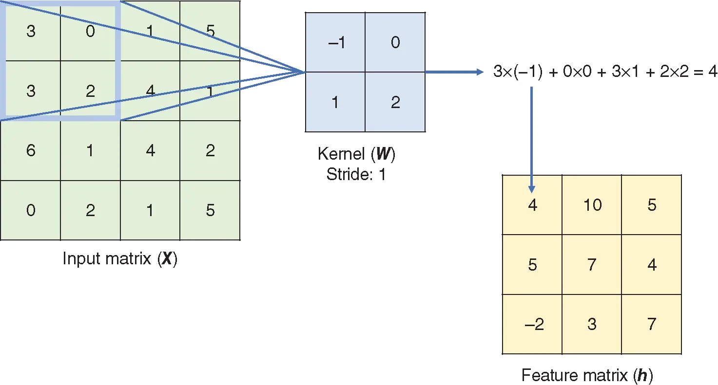
Figure 2 Convolution operation with stride size .

The convolution operation is illustrated in Figure 2. The weight matrix of the convolutional layer is usually called the kernel matrix. The kernel matrix ( ) shifts over the input matrix and performs elementwise multiplication between the kernel matrix ( ) and the covered portion of the input matrix ( ), resulting in a feature matrix ( ). The stride of the kernel matrix determines the amount of movement in each step. In the example in Figure 2, the stride size is 1, so the kernel matrix moves one unit in each step. In total, the kernel matrix shifts 9 times, resulting in a feature matrix. The stride size does not have to be 1, and a larger stride size means fewer shifts.

Another commonly used structure in a CNN is the pooling layer, which is good at extracting dominant features from the input. Two main types of pooling operation are illustrated in Figure 3. Similar to a convolution operation, the kernel shifts over the input matrix with a specified stride size. If Max Pooling is applied to the input, the maximum of the covered portion will be taken as the result. If Average Pooling is applied, the mean of the covered portion will be calculated and taken as the result. The example in Figure 3shows the result of pooling with kernel size that equals and stride that equals 1 on a input matrix.