Computational Statistics in Data Science
Здесь есть возможность читать онлайн «Computational Statistics in Data Science» — ознакомительный отрывок электронной книги совершенно бесплатно, а после прочтения отрывка купить полную версию. В некоторых случаях можно слушать аудио, скачать через торрент в формате fb2 и присутствует краткое содержание. Жанр: unrecognised, на английском языке. Описание произведения, (предисловие) а так же отзывы посетителей доступны на портале библиотеки ЛибКат.
- Название:Computational Statistics in Data Science
- Автор:
- Жанр:
- Год:неизвестен
- ISBN:нет данных
- Рейтинг книги:4 / 5. Голосов: 1
-
Избранное:Добавить в избранное
- Отзывы:
-
Ваша оценка:
Computational Statistics in Data Science: краткое содержание, описание и аннотация
Предлагаем к чтению аннотацию, описание, краткое содержание или предисловие (зависит от того, что написал сам автор книги «Computational Statistics in Data Science»). Если вы не нашли необходимую информацию о книге — напишите в комментариях, мы постараемся отыскать её.
Computational Statistics in Data Science
Computational Statistics in Data Science
Wiley StatsRef: Statistics Reference Online
Computational Statistics in Data Science
Computational Statistics in Data Science — читать онлайн ознакомительный отрывок
Ниже представлен текст книги, разбитый по страницам. Система сохранения места последней прочитанной страницы, позволяет с удобством читать онлайн бесплатно книгу «Computational Statistics in Data Science», без необходимости каждый раз заново искать на чём Вы остановились. Поставьте закладку, и сможете в любой момент перейти на страницу, на которой закончили чтение.
Интервал:
Закладка:
4.3 LeNet‐5
LeNet‐5 is a CNN introduced by LeCun et al . [8]. This is one of the earliest structures of CNNs and was initially introduced to do handwritten digit recognition on the MNIST dataset [9]. The structure is straightforward and simple to understand, and details are shown in Figure 4.
The LeNet‐5 architecture consists of seven layers, where three are convolutional layers, two are pooling layers, and two are fully connected layers. LeNet‐5 takes images of size  as input and outputs a 10‐dimensional vector as the predict scores for each class.
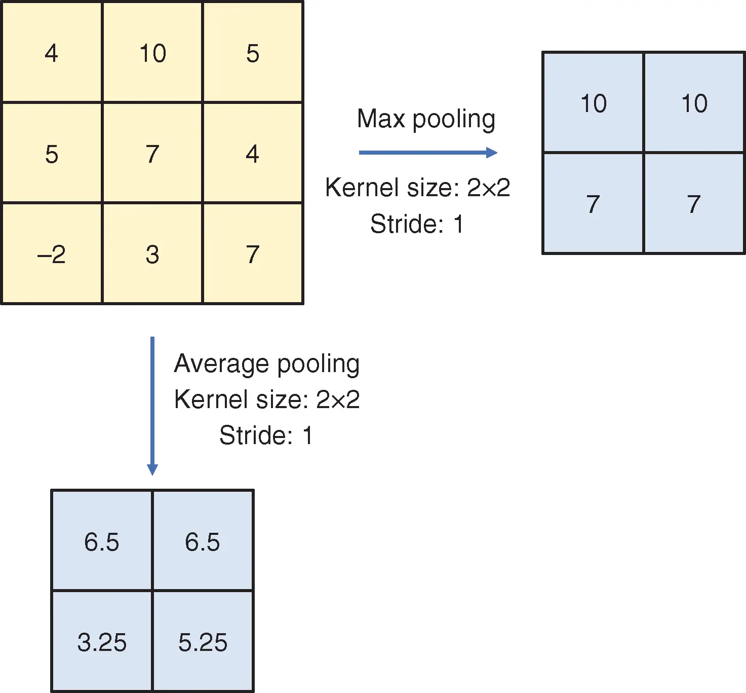
Figure 3 Pooling operation with stride size  .
.

Figure 4
LeNet‐5 of LeCun et al . [8].
Source : Modified from LeCun et al . [8].
The first layer (C1) is a convolutional layer, which consists of six kernel matrices of size  and stride 1. Each of the kernel matrices will scan over the input image and produce a feature matrix of size
  . Therefore, six different kernel matrices will produce six different feature matrices. The second layer (S2) is a Max Pooling layer, which takes the
  matrices as input. The kernel size of this pooling layer is
  , and the stride size is 2. Therefore, the outputs of this layer are six
  feature matrices.
Table 1 Connection between input and output matrices in the third layer of LeNet‐5 [8].
Source : LeCun et al . [8].
| Indices of output matrices | ||||||||||
|---|---|---|---|---|---|---|---|---|---|---|
| 1 | 1 | 5 | 6 | 7 | 10 | 11 | 12 | 13 | 15 | 16 |
| 2 | 1 | 2 | 6 | 7 | 8 | 11 | 12 | 13 | 14 | 16 |
| 3 | 1 | 2 | 3 | 7 | 8 | 9 | 12 | 14 | 15 | 16 |
| 4 | 2 | 3 | 4 | 7 | 8 | 9 | 10 | 13 | 15 | 16 |
| 5 | 3 | 4 | 5 | 8 | 9 | 10 | 11 | 13 | 14 | 16 |
| 6 | 4 | 5 | 6 | 9 | 10 | 11 | 12 | 14 | 15 | 16 |
The row names are indices of input matrices, and the second column shows indices of output matrices that are connected to the corresponding input matrix. There are  connections in total, meaning
  different kernel matrices.
The third layer (C3) is the second convolutional layer in LeNet‐5. It consists of 60 kernel matrices of size  , and the stride size 1. Therefore, the output feature matrices are of size
  . Note that the relationship between input matrices and output matrices in this layer is not fully connected. Each of the input matrices is connected to a part of the output matrices. Details of the connection can be found in Table 1. Input matrices connected to the same output matrix will be used to produce the output matrix. Take the first output matrix, which is connected to the first three input matrices, as an example. The first three input matrices will be filtered by three different kernel matrices and result in three
  feature matrices. The three feature matrices will first be added together, and then a bias is added elementwise, resulting in the first output matrix. There are 16 feature matrices of size
  produced by layer C3.
The fourth layer (S4) is a Max Pooling layer that produces 16 feature matrices with size  . The kernel size of this layer is
  , and the stride is 2. Therefore, each of the input matrices is reduced to
  . The fifth layer (C5) is the last convolutional layer in LeNet‐5. The 16 input matrices are fully connected to 120 output matrices. Since both the input matrices and kernel matrices are of size
  , the output matrices are of size
  . Therefore, the output is actually a 120‐dimensional vector. Each number in the vector is computed by applying 16 different kernel matrices on the 16 different input matrices and then combining the results and bias.
The sixth and seventh layers are fully connected layers, which are introduced in the previous section. In the sixth layer (S6), 120 input neurons are fully connected to 84 output neurons. In the last layer, 84 neurons are fully connected to 10 output neurons, where the 10‐dimensional output vector contains predict scores of each class. For the classification task, cross‐entropy loss between the model output and the label is usually used to train the model.
There are many other architectures of CNNs, such as AlexNet [10], VGG [11], and ResNet [12]. These neural networks demonstrated state‐of‐the‐art performances on many machine learning tasks, such as image classification, object detection, and speech processing.
5 Autoencoders
5.1 Introduction
An autoencoder is a special type of DNN where the target of each input is the input itself [13]. The architecture of an autoencoder is shown in Figure 5, where the encoder and decoder together form the autoencoder. In the example, the autoencoder takes a horse image as input and produces an image similar to the input image as output. When the embedding dimension is greater than or equal to the input dimension, there is a risk of overfitting, and the model may learn an identity function. One common solution is to make the embedding dimension smaller than the input dimension. Many studies showed that the intrinsic dimension of many high‐dimensional data, such as image data, is actually not truly high‐dimensional; thus, they can be summarized by low‐dimensional representations. Autoencoder summarizes the high‐dimensional data information with low‐dimensional embedding by training the framework to produce output that is similar to the input. The learned representation can be used in various downstream tasks, such as regression, clustering, and classification. Even if the embedding dimension is as small as 1, overfitting is still possible if the number of parameters in the model is large enough to encode each sample to an index. Therefore, regularization [15] is required to train an autoencoder that reconstructs the input well and learns a meaningful embedding.
Читать дальшеИнтервал:
Закладка:
Похожие книги на «Computational Statistics in Data Science»
Представляем Вашему вниманию похожие книги на «Computational Statistics in Data Science» списком для выбора. Мы отобрали схожую по названию и смыслу литературу в надежде предоставить читателям больше вариантов отыскать новые, интересные, ещё непрочитанные произведения.
![Роман Зыков - Роман с Data Science. Как монетизировать большие данные [litres]](/books/438007/roman-zykov-roman-s-data-science-kak-monetizirova-thumb.webp)


Обсуждение, отзывы о книге «Computational Statistics in Data Science» и просто собственные мнения читателей. Оставьте ваши комментарии, напишите, что Вы думаете о произведении, его смысле или главных героях. Укажите что конкретно понравилось, а что нет, и почему Вы так считаете.