Manuel Pastor - Computational Geomechanics

If complete saturation is assumed together with a linear form of the constitutive law, we can write the effective stress simply as

(3.62)

We can now reduce the governing u– p Equations (3.23)and (3.28)to the form given below

(3.63)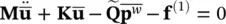

and

(3.64)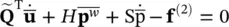

where =

(3.65)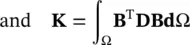

is the well‐known elastic stiffness matrix which is always symmetric in form. Sand Hare again symmetric matrices defined in (3.31)and (3.30)and is as defined in (3.29).

The overall system can be written in the terms of the variable set [ , ] Tas

(3.66)

Once again the uncoupled nature of the problem under drained condition is evident (by dropping the time derivatives) giving

(3.67)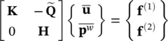

in which can be separately determined by solving the second equation. For undrained behavior , we can integrate the second equation when H= 0 and obtain an antisymmetric system which can be made symmetric by multiplying the second equation by minus unity (Zienkiewicz and Taylor 1985)

(3.68)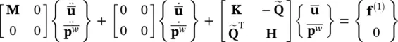

It is interesting to observe that in the steady state, we have a matrix which, in the absence of fluid compressibility, results in

(3.69)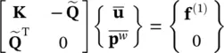

which only can have a unique solution when the number of variables n uis greater than the number of variables n p. This is one of the requirements of the patch test of Zienkiewicz et al. (1986a, 1986b) and of the Babuska‐Brezzi (Babuska 1973 and Brezzi 1974) condition.

In general, when dynamic problems are encountered in soils (or other geomaterials), the damping introduced by the plastic behavior of the material and the viscous effects of the fluid flow are sufficient to damp out any nonphysical or numerical oscillation. However, if the solutions of the problems are in the low‐strain range when the plastic hysteresis is small or when, to simplify the procedures, purely elastic behavior is assumed, it may be necessary to add system damping matrices of the form to the dynamic equations of the solid phase, i.e. changing (3.23)to

(3.70)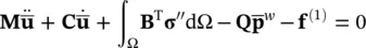

Indeed, such damping matrices have a physical significance and are always introduced in earthquake analyses or similar problems of structural dynamics. With the lack of any special information about the nature of damping, it is usual to assume the so‐called “Rayleigh damping” in which

(3.71)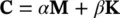

where α and β are coefficients determined by experience (see, for instance, Clough and Penzien (1975) or (1993)). In the above, Mis the same mass matrix as given in (3.24)and Kis some representative stiffness matrix of the form given in (3.47).

The equation numbers given here correspond to the ones given earlier in the text.

(3.8b)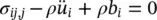

(3.9b)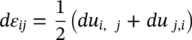

Noting that the engineering shear strain dγ xyis defined as:

Equation (3.10)is scalar

(3.11b)

(3.12b)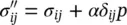

Equation (3.13)is scalar.

Equation (3.14)is scalar.

(3.15b)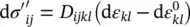

Equation (3.16)is scalar

(3.17b)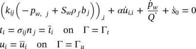

and

(3.18b)