Manuel Pastor - Computational Geomechanics

(3.32)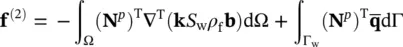

where Q *is defined as in (2.30c), i.e.

(3.33)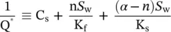

and C S, S w, C wand kdepend on p w.

To complete the numerical solution, it is necessary to integrate the ordinary differential Equations (3.23), (3.27), and (3.28)in time by one of the many available schemes. Although there are many multistep methods available (see, e.g., Wood 1990), they are inconvenient as most of them are not self‐starting and it is more difficult to incorporate restart facilities which are required frequently in practical analyses. On the other hand, the single‐step methods handle each step separately and there is no particular change in the algorithm for such restart requirements.

Two similar, but distinct, families of single‐step methods evolved separately. One is based on the finite element and weighted residual concept in the time domain and the other based on a generalization of the Newmark or finite difference approach. The former is known as the SSpj – Single Step p thorder scheme for j thorder differential equation ( p ≥ j ). This was introduced by Zienkiewicz et al. (1980b, 1984) and extensively investigated by Wood (1984a, 1984b, 1985a, 1985b). The SSpj scheme has been used successfully in SWANDYNE‐I (Chan, 1988). The later method, which was adopted in SWANDYNE‐II (Chan 1995) was an extension to the original work of Newmark (1959) and is called Beta‐m method by Katona (1985) and renamed the Generalized Newmark (GNpj) method by Katona and Zienkiewicz (1985). Both methods have similar or identical stability characteristics. For the SSpj, no initial condition, e.g. acceleration in dynamical problems, or higher time derivatives are required. On the other hand, however, all quantities in the GNpj method are defined at a discrete time station, thus making transfer of such quantities between the two equations easier to handle. Here we shall use the later (GNpj) method, exclusively, due to its simplicity.

In all time‐stepping schemes, we shall write a recurrence relation linking a known value ϕ n(which can either be the displacement or the pore water pressure), and its derivatives , ,… at time station t nwith the values of Φ n+1, , ,…, which are valid at time t n+ Δ t and are the unknowns. Before treating the ordinary differential equation system (3.23), (3.27), and (3.28), we shall illustrate the time‐stepping scheme on the simple example of (3.6) by adding a forcing term:

(3.34)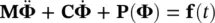

From the initial conditions, we have the known values of Φ n, . We assume that the above equation has to be satisfied at each discrete time, i.e. t nand t n+1. We can thus write:

(3.35)

and

(3.36)

From the first equation, the value of the acceleration at time t ncan be found and this solution is required if the initial conditions are different from zero.

The link between the successive values is provided by a truncated series expansion taken in the simplest case as GN22 as Equation (3.34)is a second‐order differential equation j and the minimum order of the scheme required is then two: as ( p ≥ j )

(3.37)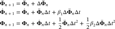

Alternatively, a higher order scheme can be chosen such as GN32 and we shall have:

(3.38)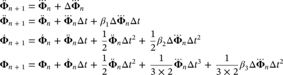

In this case, an extra set of equations is required to obtain the value of the highest time derivatives. This is provided by differentiating (3.35)and (3.36).

(3.39)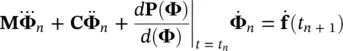

and

(3.40)

In the above equations, the only unknown is the incremental value of the highest derivative and this can be readily solved for.

Returning to the set of ordinary differential equations we are considering here, i.e. (3.23), (3.27), and (3.28)and writing (3.23)and (3.28)at the time station t n+1, we have:

(3.41)

(3.42)

assuming that (3.27)is satisfied.

Using GN22 for the displacement parameters and GN11 for the pore pressure parameter w, we write:

(3.43a)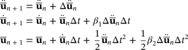

and

(3.43b)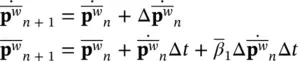

where and are as yet undetermined quantities. The parameters β 1, β 2, and are usually chosen in the range of 0 to 1. For β 2= 0 and = 0, we shall have an explicit form if both the mass and damping matrices are diagonal. If the damping matrix is non‐diagonal, an explicit scheme can still be achieved with β 1= 0, thus eliminating the contribution of the damping matrix. The well‐known central difference scheme is recovered from (3.41)if β 1= 1/2, β 2= 0 and this form with an explicit and implicit scheme has been considered in detail by Zienkiewicz et al. (1982) and Leung (1984). However, such schemes are only conditionally stable and for unconditional stability of the recurrence scheme, we require