Manuel Pastor - Computational Geomechanics

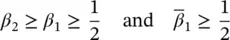
The optimal choice of these values is a matter of computational convenience, the discussion of which can be found in literature. In practice, if the higher order accurate “trapezoidal” scheme is chosen with β 2= β 1= 1/2 and = 1/2, numerical oscillation may occur if no physical damping is present. Usually, some algorithmic (numerical) damping is introduced by using such values as

or

Dewoolkar (1996), using the computer program SWANDYNE II in the modelling of a free‐standing retaining wall, reported that the first set of parameters led to excessive algorithmic damping as compared to the physical centrifuge results. Therefore, the second set was used and gave very good comparisons. However, in cases involving soil, the physical damping (viscous or hysteretic) is much more significant than the algorithmic damping introduced by the time‐stepping parameters and the use of either sets of parameters leads to similar results.

Inserting the relationships (3.43) into Equations (3.41)and (3.42)yields a general nonlinear equation set in which only and remain as unknowns.

This set can be written as

(3.44a)

(3.44b)

where and can be evaluated explicitly from the information available at time t nand

(3.45)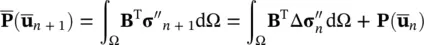

In this, must be evaluated by integrating (3.27)as the solution proceeds. The values of n+1and n+1at the time t n+1are evaluated by Equation (3.43).

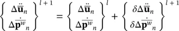
The equation will generally need to be solved by a convergent, iterative process using some form of Newton–Raphson procedure typically written as

(3.46a)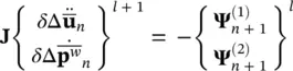

where 1 is the iteration number and

The Jacobian matrix can be written as

(3.47)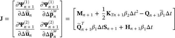

where

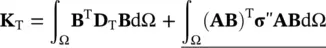
which are the well‐known expressions for tangent stiffness matrix. The underlined term corresponds to the “initial stress” matrix evaluated in the current configuration as a result of stress rotation defined in (2.5).

Two points should be made here:

1 that in the linear case, a single “iteration” solves the problem exactly

2 that the matrix can be made symmetric by a simple scalar multiplication of the second row (provided KT is itself symmetric).

In practice, it is found that the use of various approximations of the matrix Jis advantageous such as, for instance, the use of “secant” updates (see, for instance, Crisfield (1979), Matthies, and Strang (1979) and Zienkiewicz et al (2013).

A particularly economical computation form is given by choosing β 2= 0 and representing matrix Min a diagonal form. This explicit procedure was first used by Leung (1984) and Zienkiewicz et al. (1980a). It is, however, only conditionally stable and is efficient only for phenomena of short duration.

The process of the time‐domain solution of (3.44) can be amended to that of successive separate solutions of the time equations for variables and , respectively, using an approximation for the remaining variable. Such staggered procedures, if stable, can be extremely economical as shown by Park and Felippa (1983) but the particular system of equations presented here needs stabilization. This was first achieved by Park (1983) and, later, a more effective form was introduced by Zienkiewicz et al. (1988).

Special cases of solution are incorporated in the general solution scheme presented here without any modification and indeed without loss of computational efficiency.

Thus, for static or quasi‐static, problems, it is merely necessary to put M= 0 and immediately the transient consolidation equation is available. Here time is still real and we have omitted only the inertia effects (although with implicit schemes, this a priori assumption is not necessary and inertia effects will simply appear as negligible without any substantial increase of computation). In pure statics, the time variable is still retained but is then purely an artificial variable allowing load incrementation.

In static or dynamic undrained analysis, the permeability (and compressibility) matrices are set to zero, i.e. H· f (2)= 0, and usually S= 0 resulting in a zero‐matrix diagonal term in the Jacobian matrix of Equation (3.47).

The matrix to be solved in such a limiting case is identical to that used frequently in the solution of problems of incompressible elasticity or fluid mechanics and, in such studies, places limitations on the approximating functions N uand N pused in (3.19)if the Babuska–Brezzi (Babuska 1971, 1973, Brezzi 1974) convergence conditions or their equivalent (Zienkiewicz et al. 1986b) are to be satisfied. Until now, we have not referred to any particular element form, and, indeed, a wide choice is available to the user if the limiting (undrained) condition is never imposed. Due to the presence of first derivatives in space in all the equations, it is necessary to use “ C 0‐continuous” interpolation functions and Figure 3.2shows some elements incorporated in the formulation. The form of most of the elements used satisfies the necessary convergence criteria of the undrained limit (Zienkiewicz 1984). Though the bi‐linear u and p quadrilateral does not, it is, however, useful when the permeability is sufficiently large.