Manuel Pastor - Computational Geomechanics
Здесь есть возможность читать онлайн «Manuel Pastor - Computational Geomechanics» — ознакомительный отрывок электронной книги совершенно бесплатно, а после прочтения отрывка купить полную версию. В некоторых случаях можно слушать аудио, скачать через торрент в формате fb2 и присутствует краткое содержание. Жанр: unrecognised, на английском языке. Описание произведения, (предисловие) а так же отзывы посетителей доступны на портале библиотеки ЛибКат.

- Название:Computational Geomechanics
- Автор:
- Жанр:
- Год:неизвестен
- ISBN:нет данных
- Рейтинг книги:4 / 5. Голосов: 1
-
Избранное:Добавить в избранное
- Отзывы:
-
Ваша оценка:
Computational Geomechanics: краткое содержание, описание и аннотация
Предлагаем к чтению аннотацию, описание, краткое содержание или предисловие (зависит от того, что написал сам автор книги «Computational Geomechanics»). Если вы не нашли необходимую информацию о книге — напишите в комментариях, мы постараемся отыскать её.
Computational Geomechanics: Theory and Applications, Second Edition
Computational Geomechanics — читать онлайн ознакомительный отрывок
Ниже представлен текст книги, разбитый по страницам. Система сохранения места последней прочитанной страницы, позволяет с удобством читать онлайн бесплатно книгу «Computational Geomechanics», без необходимости каждый раз заново искать на чём Вы остановились. Поставьте закладку, и сможете в любой момент перейти на страницу, на которой закончили чтение.
Интервал:
Закладка:
where Dis the tangent matrix dependent on the state variables and history and ε 0corresponds to thermal and creep strains.
The main variables of the problem are thus uand p w. The effective stresses are determined at any stage by a sum of all previous increments and the value of p wdetermines the parameters S w(saturation) and χ w(effective area). On occasion, the approximation
(3.16) 
can be used.
An additional equation is supplied by the mass conservation coupled with fluid momentum balance. This is conveniently given by (2.33b)which can be written as
(3.17) 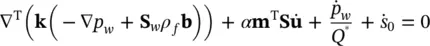
with k= k( S w).
The contribution of the solid acceleration is neglected in this equation. Its inclusion in the equation will render the final equation system nonsymmetric (see Leung 1984) and the effect of this omission has been investigated in Chan (1988) who found it to be insignificant. However, it has been included in the force term of the computer code SWANDYNE‐II (Chan 1995) although it is neglected in the left‐hand side of the final algebraic equation when the symmetric solution procedure is used.
The above set defines the complete equation system for solution of the problem defined providing the necessary boundary conditions have been specified as in (2.18)and (2.19), i.e.
(3.18) 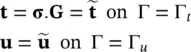
and
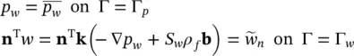
Assuming isotropic permeability, the above equation becomes
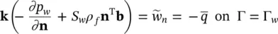
where  is the influx, i.e. having an opposite sign to the outflow
  .
.
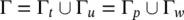
The total boundary Γ is the union of its components, i.e.
3.2.2 Discretization of the Governing Equation in Space
The spatial discretization involving the variables uand p wis achieved by suitable shape (or basis) functions, writing
(3.19) 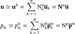
Note that the nodal values of the pore pressures are indicated with a superscript.
We assume here that the expansion is such that the strong boundary conditions (3.18)are satisfied on Γ uand Γ pautomatically by a suitable prescription of the (nodal) parameters. As in most other finite element formulations, the natural boundary condition will be obtained by integrating the weighted equation by parts.
To obtain the first equation discretized in space, we premultiply (3.8)by ( N u) Tand integrate the first term by parts (see for details Zienkiewicz et al (2013) or other texts) giving:
(3.20) 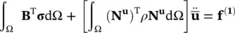
where the matrix Bis given as
(3.21) 
and the “load vector” f (1), equal in number of components to that of vector  contains all the effects of body forces, and prescribed boundary tractions, i.e.
(3.22) 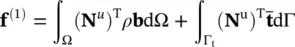
At this stage, it is convenient to introduce the effective stress see (3.12)now defined to allow for effects of incomplete saturation as
(3.23) 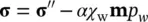
The discrete, ordinary differential equation now becomes
(3.24) 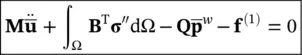
where
(3.25) 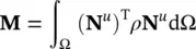
is the MASS MATRIX of the system and
(3.26) 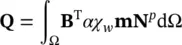
is the coupling matrix‐linking equation (3.23)and those describing the fluid conservation, and
(3.22 \ bis) 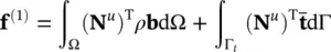
The computation of the effective stress proceeds incrementally as already indicated in the usual way and now (3.15)can be written in discrete form:
(3.27) 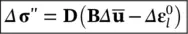
where, of course, Dis evaluated from appropriate state and history parameters.
Finally, we discretize Equation (3.17)by pre‐multiplying by ( N p) Tand integrating by parts as necessary. This gives the ordinary differential equation
(3.28) 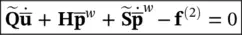
where the various matrices are as defined below
(3.29) 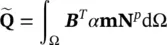
(3.30) 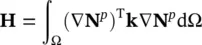
(3.31) 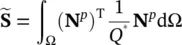
Интервал:
Закладка:
Похожие книги на «Computational Geomechanics»
Представляем Вашему вниманию похожие книги на «Computational Geomechanics» списком для выбора. Мы отобрали схожую по названию и смыслу литературу в надежде предоставить читателям больше вариантов отыскать новые, интересные, ещё непрочитанные произведения.


Обсуждение, отзывы о книге «Computational Geomechanics» и просто собственные мнения читателей. Оставьте ваши комментарии, напишите, что Вы думаете о произведении, его смысле или главных героях. Укажите что конкретно понравилось, а что нет, и почему Вы так считаете.