Manuel Pastor - Computational Geomechanics

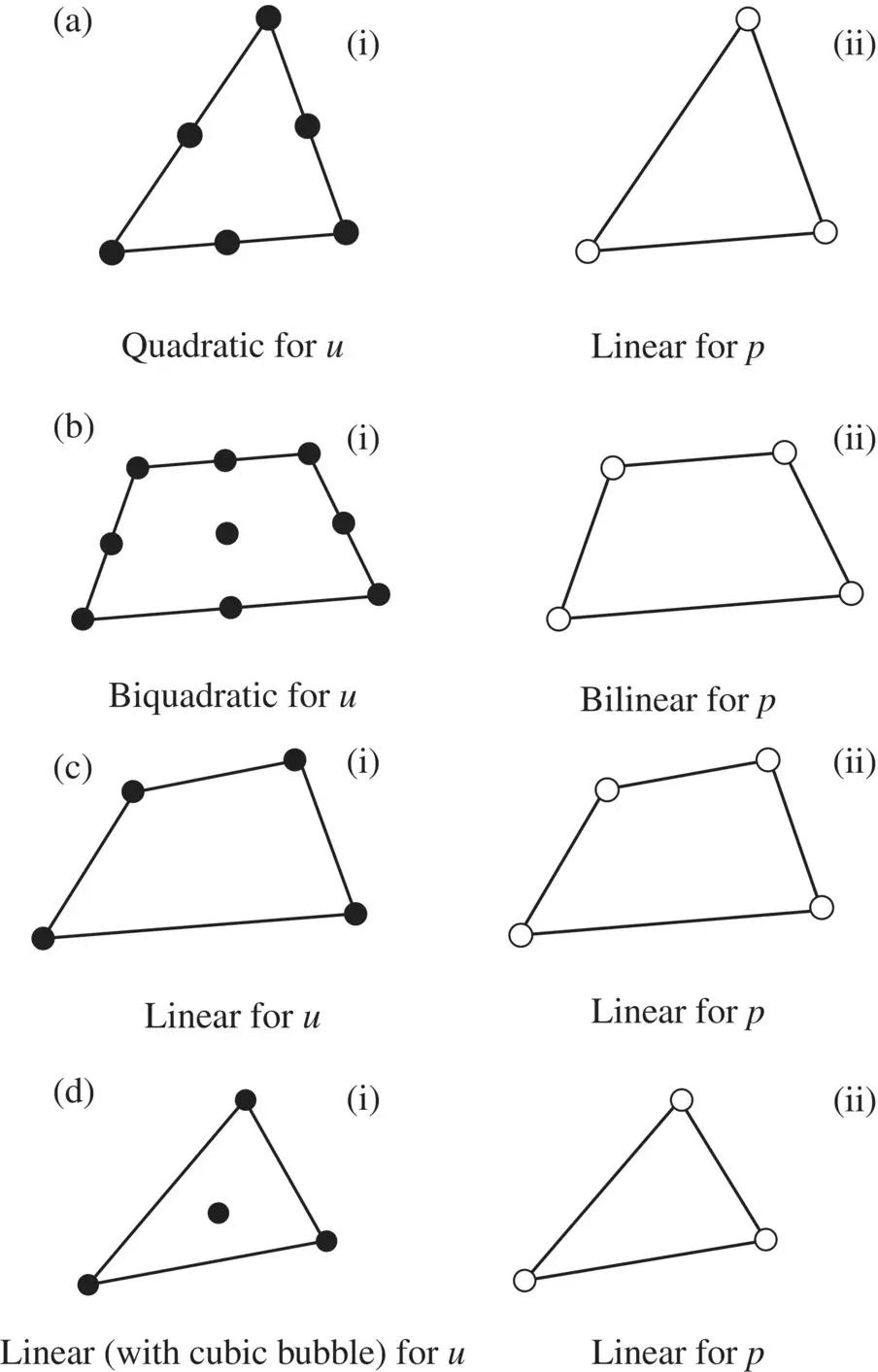
Figure 3.2 Elements used for coupled analysis, displacement ( u ) and pressure ( p ) formulation: (a) (i) quadratic for u ; (ii) linear for p ; (b) (i) biquadratic for u ; (ii) bilinear for p : (c) (i) linear for u ; (ii) linear for p : (d) (i) linear (with cubic bubble) for u ; (ii) linear for Element ( c ) is not fully acceptable at incompressible–undrained limits.

We shall return to this problem in Chapter 5where a modification is introduced allowing the same interpolations to be used for both u and p .

In that chapter, we shall discuss a possible amendment to the code permitting the use of identical u ‐p interpolation even in incompressible cases.

We note that all computations start from known values of and wpossibly obtained as the result of static computations by the same program in a manner which will be explained in the next Section 3.2.4. The incremental computation allows the various parameters, dependent on the solution history, to be updated.

Thus, for known Δ increment, the Δ σ ″are evaluated by using an appropriate tangent matrix Dand an appropriate stress integration scheme.

Further, we note that if p w≥ 0 (full saturation, described in Section 2.2of the previous chapter), then we have

and the permeability remains at its saturated value

However, when negative pressures are reached, i.e. when p w< 0, the values of S w, χ w, and k have to be determined from appropriate formulae or graphs.

As explained in the previous Section 3.2.3, the computation always proceeds in an incremental manner and in the u‐ p form in general, the explicit time stepping is not used as its limitation is very serious. Invariably, the algorithm is applied here to the unconditionally stable, implicit form and the equation system given by the Jacobian of (3.46) with variables Δ and Δ needs to be solved at each time step.

With unconditional stability of the implicit scheme, the only limitation on the length of the time step is the accuracy achievable. Clearly, in the dynamic earthquake problem, short time steps will generally be used to follow the time characteristic of the input motion. In the examples that we shall give later, we shall frequently use simply the time interval Δ t = 0.02 s which is the interval used usually in earthquake records.

However, once the input motion has ceased and its record no longer has to be followed, a much longer length of time step could be adopted. Indeed, after the passage of the earthquake, the remaining motion is caused by something resembling a consolidation process which has a slower response allowing longer time steps to be used.

The length of the time step based on accuracy considerations was first discussed in Zienkiewicz et al. (1984), Zienkiewicz and Shiomi (1984), and, later, by Zienkiewicz and Xie (1991), and Bergan and Mollener (1985).

The simplest process is that which considers the expansion for such a variable as ugiven by (3.43) and its comparison with a Taylor series expansion.

Clearly, for a scalar variable u , the error term is given by the first omitted terms of the Taylor expansion, i.e., in scalar values

(3.48)

Using an approximation of this third derivative shown below

(3.49)

we have

(3.50)

For a vector variable u, we must consider its L 2norm, i.e.

(3.51)

and we can limit the error to

(3.52)

This limit was reestablished later by Zienkiewicz and Xie (1991) who replaced the leading coefficient of (3.52)as a result of a more detailed analysis by

(3.53)

Whatever the form of error estimator adopted, the essence of the procedure is identical and this is given by establishing a priori some limits or tolerance which must not be exceeded, and modifying the time steps accordingly.

In the above, we have considered only the error in one of the variables, i.e. u but, in general, this suffices for quite a reasonable error control.

The tolerance is conveniently chosen as some percentage η of the maximum value of norm ‖ u‖ 2recorded. Thus, we write

(3.54)

with some minimum specified.

The time step can always be adjusted during the process of computation noting, however, not to change the length of the time step by more than a factor of 2 or ½, otherwise unacceptable oscillations may arise.

The most common way of solving the coupled system of equations is the monolithic scheme where both the coupled equations are solved simultaneously at each time step as discussed above. However, also splitting solutions are possible where the two (or three) equations are solved separately at each time step. To conserve the coupled nature of the problem, iterations within each time step are necessary even in the linear case. The reason for applying partitioned solutions may be the fact that solvers for the solid and fluid fields are already at hand so that only the interaction has to be taken into account. This type of solution procedure is extensively investigated for the dynamic case by Markert et al. (2010) and, as already mentioned, by Park and Felippa (1983), Park (1983), and Zienkiewicz et al. (1988). A splitting procedure will be used in Section 5.5 both for the dynamic case and consolidation allowing for same interpolation for both uand p . Partitioned solutions are quite common in consolidation and have been extensively treated in Lewis and Schrefler (1998). From the investigation of the iteration convergence within a time step, Turska and Schrefler (1993) found the existence of a lower limit for Δ t/h 2which means that it is not always possible to decrease Δ t without also decreasing the mesh size h . Such a limit was also found by Murthy et al. (1989) for Poisson‐type equations and by Rank et al. (1983) for transient finite element analyses by invoking the discrete maximum principle.