Richard J. Rossi - Applied Biostatistics for the Health Sciences
Здесь есть возможность читать онлайн «Richard J. Rossi - Applied Biostatistics for the Health Sciences» — ознакомительный отрывок электронной книги совершенно бесплатно, а после прочтения отрывка купить полную версию. В некоторых случаях можно слушать аудио, скачать через торрент в формате fb2 и присутствует краткое содержание. Жанр: unrecognised, на английском языке. Описание произведения, (предисловие) а так же отзывы посетителей доступны на портале библиотеки ЛибКат.

- Название:Applied Biostatistics for the Health Sciences
- Автор:
- Жанр:
- Год:неизвестен
- ISBN:нет данных
- Рейтинг книги:3 / 5. Голосов: 1
-
Избранное:Добавить в избранное
- Отзывы:
-
Ваша оценка:
Applied Biostatistics for the Health Sciences: краткое содержание, описание и аннотация
Предлагаем к чтению аннотацию, описание, краткое содержание или предисловие (зависит от того, что написал сам автор книги «Applied Biostatistics for the Health Sciences»). Если вы не нашли необходимую информацию о книге — напишите в комментариях, мы постараемся отыскать её.
APPLIED BIOSTATISTICS FOR THE HEALTH SCIENCES Applied Biostatistics for the Health Sciences
Applied Biostatistics for the Health Sciences
Applied Biostatistics for the Health Sciences — читать онлайн ознакомительный отрывок
Ниже представлен текст книги, разбитый по страницам. Система сохранения места последней прочитанной страницы, позволяет с удобством читать онлайн бесплатно книгу «Applied Biostatistics for the Health Sciences», без необходимости каждый раз заново искать на чём Вы остановились. Поставьте закладку, и сможете в любой момент перейти на страницу, на которой закончили чтение.
Интервал:
Закладка:
The coefficient of variation compares the size of the standard deviation with the size of the mean. When the coefficient of variation is small, this means that the variability in the population is relatively small compared to the size of the mean of the population. On the other hand, when the coefficient of variation is large, this indicates that the population varies greatly relative to the size of the mean. The standard for what is a large coefficient of variation differs from one discipline to another, and in some disciplines a coefficient of variation of less than 15% is considered reasonable, and in other disciplines larger or smaller cutoffs are used.
Because the standard deviation and the mean have the same units of measurement, the coefficient of variation is a unitless parameter. That is, the coefficient is unaffected by changes in the units of measurement. For example, if a variable X is measured in inches and the coefficient of variation is CV = 2, then coefficient of variation will also be 2 when the units of measurement are converted to centimeters. The coefficient of variation can also be used to compare the relative variability in two different and unrelated populations; the standard deviation can only be used to compare the variability in two different populations based on similar variables.
Example 2.18
Use the means and standard deviations given in Table 2.6for the three variables that were measured on a population to answer the following questions:
Table 2.6 The Means and Standard Deviations for Three Different Variables
| Variable | µ | σ |
|---|---|---|
| I | 100 | 25 |
| II | 10 | 5 |
| III | 0.10 | 0.05 |
1 Determine the value of the coefficient of variation for population I.
2 Determine the value of the coefficient of variation for population II.
3 Determine the value of the coefficient of variation for population III.
4 Compare the relative variability of each variable.
Solutions
1 The value of the coefficient of variation for population I is CVI=25100=0.25.
2 The value of the coefficient of variation for population II is CVII=510=0.5.
3 The value of the coefficient of variation for population III is CVIII=0.050.10=0.5.
4 Populations II and III are relatively more variable than population I even though the standard deviations for populations II and III are smaller than the standard deviation of population I. Populations II and III have the same amount of relative variability even though the standard deviation of population III is one-hundredth that of population II.
The previous example illustrates how comparing the absolute size of the standard deviation is relevant only when comparing similar variables. Also, interpreting the size of a standard deviation should take into account the size of a typical value in a population. For example, a standard deviation of σ = 0.01 might appear to be a small standard deviation; however, if the mean was µ = 0.006, then this would be a very large standard deviation (CV =167%); on the other hand, if the mean was µ = 5.2, then σ = 0.01 would be a small standard deviation (CV =0.2%).
2.2.7 Parameters for Bivariate Populations
In most biomedical research studies, there are many variables that will be recorded on each individual in the study. A multivariate distribution can be formed by jointly tabulating, charting, or graphing the values of the variables over the N units in the population. For example, the bivariate distribution of two variables, say X and Y , is the collection of the ordered pairs

These N ordered pairs form the units of the bivariate distribution of X and Y and their joint distribution can be displayed in a two-way chart, table, or graph.
When the two variables are qualitative, the joint proportions in the bivariate distribution are often denoted by p ab, where

The joint proportions in the bivariate distribution are then displayed in a two-way table or two-way bar chart. For example, according to the American Red Cross, the joint distribution of blood type and Rh factor is given in Table 2.7and presented as a bar chart in Figure 2.21.
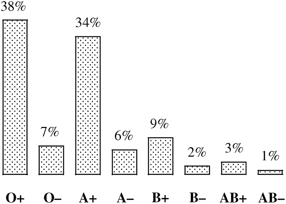
Figure 2.21 The joint distribution of blood type and Rh factor according to the American Red Cross.
Table 2.7 The Distribution of Blood Type by Rh Factor According to the American Red Cross
| Blood Type | Rh Factor | |
|---|---|---|
| + | − | |
| O | 38% | 7% |
| A | 34% | 6% |
| B | 9% | 2% |
| AB | 3% | 1% |
In a bivariate distribution where one of the variables is quantitative and the other is qualitative, the best way to graphically present the distribution is to separate the distribution into subpopulations according to the values of the qualitative distribution. For example, if W=the weight of anindividual and G=the sex of an individual, then the best way to present the bivariate distribution of weight and gender is to present the two subpopulations separately as shown in Figure 2.22.
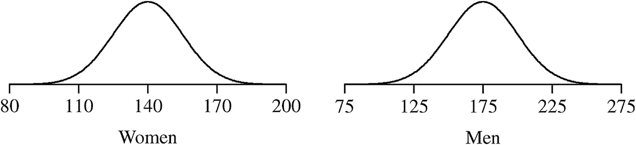
Figure 2.22 The distribution weight for the subpopulations of mean and women.
In a multivariate population, the subpopulations remain important, and the individual subpopulation proportions, percentiles, mean, median, modes, standard deviation, variance, interquartile range are important parameters that can still be used to summarize each of the subpopulations.
In a bivariate distribution where both of the variables are quantitative, a three-dimensional graph can be used to represent the joint distribution of the variables. The joint distribution is displayed as a three-dimensional probability density graph with one axis for each of the variables and the third axis representing the joint density at each pair (X,Y); however, three-dimensional density plots are sometimes difficult to interpret. An example of a three-dimensional density plot is given in Figure 2.23.
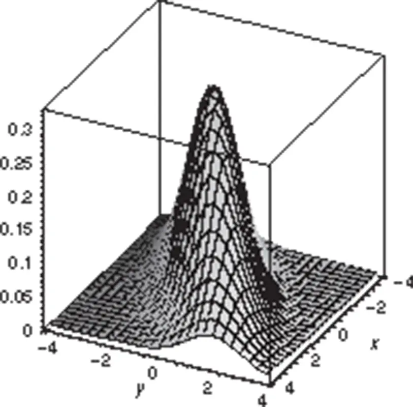
Figure 2.23 A density plot for a bivariate distribution.
To summarize the bivariate distribution of two quantitative variables, proportions, percentiles, mean, median, mode, standard deviation, variance, and interquartile range can be computed for each variable. In a bivariate distribution, the parameters associated with each separate variable are distinguished from each other by the use of subscripts. For example, if the two variables are labeled X and Y , then the mean, median, mode, standard deviation, variance, and interquartile range of the population associated with the variable X will be denoted by
Читать дальшеИнтервал:
Закладка:
Похожие книги на «Applied Biostatistics for the Health Sciences»
Представляем Вашему вниманию похожие книги на «Applied Biostatistics for the Health Sciences» списком для выбора. Мы отобрали схожую по названию и смыслу литературу в надежде предоставить читателям больше вариантов отыскать новые, интересные, ещё непрочитанные произведения.


Обсуждение, отзывы о книге «Applied Biostatistics for the Health Sciences» и просто собственные мнения читателей. Оставьте ваши комментарии, напишите, что Вы думаете о произведении, его смысле или главных героях. Укажите что конкретно понравилось, а что нет, и почему Вы так считаете.