Richard J. Rossi - Applied Biostatistics for the Health Sciences

Even though the mean, median, and mode of these two populations are the same, clearly, population I is much more spread out than population II. The density of population II is greater at the mean, which means that population II is more concentrated at this point than population I.

When describing the typical values in the population, the more variation there is in a population the harder it is to measure the typical value, and just as there are several ways of measuring the center of a population there are also several ways to measure the variation in a population. The three most commonly used parameters for measuring the spread of a population are the variance , standard deviation , and interquartile range . For a quantitative variable X

the variance of a population is defined to be the average of the squared deviations from the mean and will be denoted by σ2 or Var(X). The variance of a variable X measured on a population consisting of N units is

the standard deviation of a population is defined to be the square root of the variance and will be denoted by σ or SD(X).

the interquartile range of a population is the distance between the 25th and 75th percentiles and will be denoted by IQR.

Note that each of these measures of spread is a positive number except in the rare case when there is absolutely no variation in the population, in which case they will all be equal to 0. Furthermore, the larger each of these values is the more variability there is in the population. For example, for the two populations in Figure 2.16 the standard deviation of population I is larger than the standard deviation of population II.

Because the standard deviation is the square root of the variance, both σ and σ 2contain equivalent information about the variation in a population. That is, if the variance is known, then so is the standard deviation and vice versa. For example, if Var(X)=σ2=25, then the standard deviation is σ=25=5, and if SD(X)=σ=20, then Var(X)=σ2=202=400. The standard deviation is generally used for describing the variation in a population because the units of the standard deviation are the same as the units of the variable; the units of the variance are the units of the variable squared. Also, the standard deviation is roughly the size of a typical deviation from the mean of the population. For example, if X is a variable measured in cubic centimeters (cc), then the standard deviation is also measured in cc’s but the variance will be measured in cc2 units.

The interquartile range also measures the variability in a population by measuring the distance between the first and third quartiles (i.e., the 25th and 75th percentiles), and therefore, the interquartile range measures the distance over which the middle 50% of the population lies. The larger IQR is, the wider the range in which the middle 50% of the population lies. Figure 2.17 shows the relationship between the IQR and the quartiles of a population.

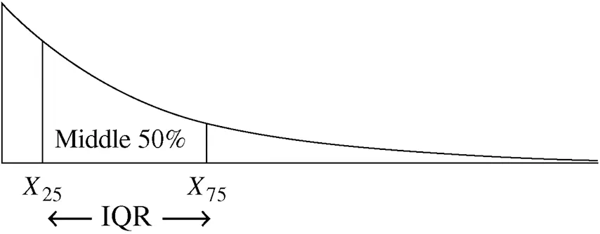
Figure 2.17 IQR is the distance between X 75and X 25.

Like the median, the interquartile range is unaffected by the extremes in a population. On the other hand, the standard deviation and variance are heavily influenced by the extremes in a population. The shape of the distribution influences the parameters of a distribution and dictates which parameters provide meaningful descriptions of the characteristics of a population. However, for a mound-shaped distribution, the standard deviation and interquartile range are closely related with σ≈0.75⋅ IQR.

Example 2.17

Consider the two populations listed below that were used in Example 2.14.

Again, these two populations are identical except for their largest values, 67 and 670. In Example 2.17, the mean values of populations 1 and 2 were found to be μ1=33.23 and μ2=79.63. The variances of these two populations are σ12=134.7 and σ22=31498.4, and the standard deviations are σ1=134.7=11.6 and σ2=31498.4=177.5. By changing the maximum value in the population from 67 to 670, the standard deviation increased by a factor of 15. In both populations, the 25th and 75th percentiles are 26 and 37, respectively, and thus, the interquartile range for both populations is IQR =37−26=11.

For mound-shaped distributions, the standard deviation is a good measure of spread, and the mean and standard deviation can be used to summarize the distribution of a mound-shaped distribution reasonably well. The Empirical Rules , which are given below, illustrate how the mean and standard deviation can be used to summarize the percentage of the population units lying within one, two, or three standard deviations of the mean. The empirical rules are presented in Figures 2.18–2.20.

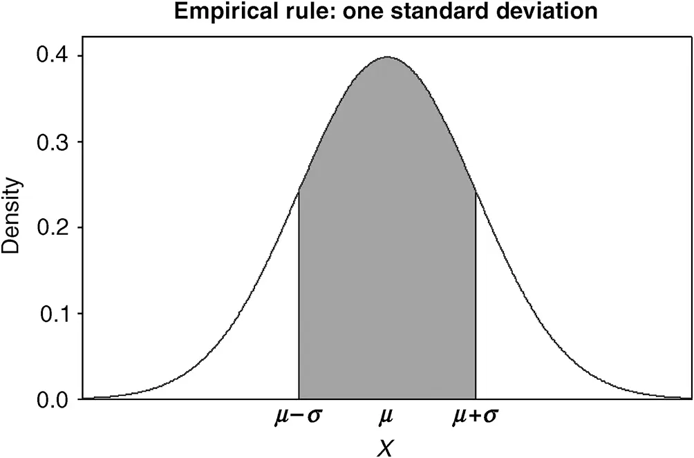
Figure 2.18 The one-standard deviation empirical rule; roughly 68% of a mound-shaped distribution lies between the values μ−σ and μ+σ.

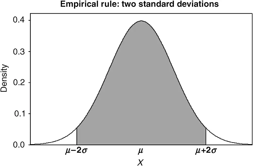
Figure 2.19The two-standard deviation empirical rule; roughly 95% of a mound-shaped distribution lies between the values μ−2σ and μ+2σ.

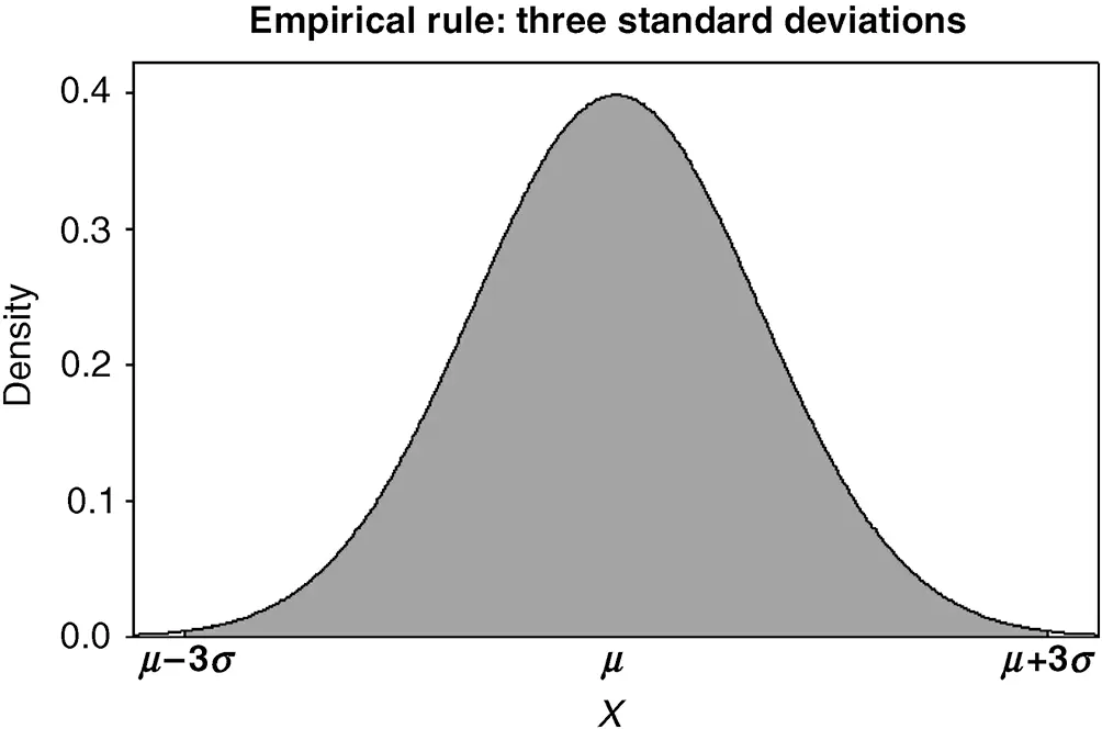
Figure 2.20 The three-standard deviation empirical rule; roughly 99% of a mound-shaped distribution lies between the values μ−3σ and μ+3σ.

For populations having mound-shaped distributions,

1 Roughly 68% of all of the population values fall within 1 standard deviation of the mean. That is, roughly 68% of the population values fall between the values μ−σ and μ+σ.

2 Roughly 95% of all the population values fall within 2 standard deviations of the mean. That is, roughly 95% of the population values fall between the values μ−2σ and μ+2σ.

3 Roughly 99% of all the population values fall within 3 standard deviations of the mean. That is, roughly 99% of the population values fall between the values μ−3σ and μ+3σ.

The standard deviations of two populations resulting from measuring the same variable can be compared to determine which of the two populations is more variable. That is, when one standard deviation is substantially larger than the other (i.e., more than two times as large), then clearly the population with the larger standard deviation is much more variable than the other. It is also important to be able to determine whether a single population is highly variable or not. A parameter that measures the relative variability in a population is the coefficient of variation . The coefficient of variation will be denoted by CV and is defined to be

The coefficient of variation is also sometimes represented as a percentage in which case