Richard J. Rossi - Applied Biostatistics for the Health Sciences

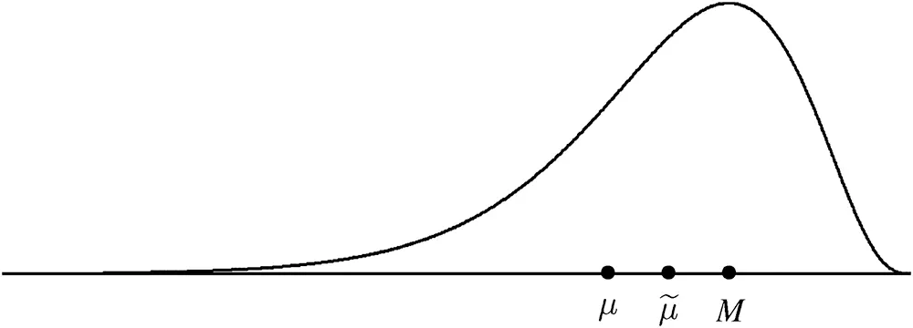
Figure 2.13 The relationships between μ,μ~, and M for a long-tail left distribution.

In general, the mean is the most commonly used measure of centrality and is a good measure of the typical value in the population as long as the distribution does not have an extremely long tail or multiple modes. For long-tailed distributions, the mean is pulled out toward the extreme tail, and in this case it is better to use the median or mode to describe the typical value in the population. Furthermore, since the median of a population is based on the middle values in the population, it is not influenced at all by the length of the tails.

Example 2.14

Consider the two populations that are listed below.

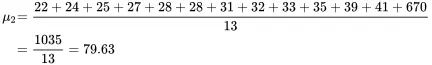
These two populations are identical except for their largest values, 67 and 670. For population 1, the mean is

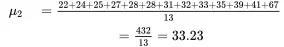
Now, because there are 11 units in population 1, the median is the sixth observation in the ordered list of population values. Thus, the median is 28. For population 2, the mean is

Since there are also 11 units in population 2, the median is also the sixth observation in the ordered list of population values. Thus, the median of population 2 is also 28.

Note that the mean of population 2 is more than twice the mean of population 1 even though the populations are identical except for their single largest values. The medians of these two populations are identical because the median is not influenced by extreme values in a population. In population 1, both the mean and median are representative of the central values of the population. In population 2, none of the population units is near the mean value, which is 79.63. Thus, the mean does not represent the value of a typical unit in population 2. The median does represent a fairly typical value in population 2 since all but one of the values in population 2 are relatively close to the value of the median.

The previous example illustrates the sensitivity of the mean to the extremes in a long-tailed distribution. Thus, in a distribution with an extremely long tail to the right or left, the mean will often be less representative than the median for describing the typical values in the population.

Recall that a multi-modal distribution generally indicates there are distinct subpopulations and the subpopulations should be described separately. When the population consists of well-defined subpopulations, the mean, median, and mode of each subpopulation should be the parameters of interest rather than the mean, median, and mode of the overall population. Furthermore, in a study with a response variable and an explanatory variable, the mean of the subpopulation of response values for a particular value of the explanatory variable is called a conditional mean and will be denoted by μY|X. Conditional means are often modeled as functions of an explanatory variable. For example, if the response variable is the weight of a 10-year-old child and the explanatory variable is the height of the child, then the distribution of weights conditioned on height is a conditional distribution. In this case, the mean weight of the conditional distributions would be a conditional mean and could be modeled as a function of the explanatory variable height.

Example 2.15

The distribution of the age of onset of obsessive compulsive disorder given in Figure 2.14 is bimodal indicating there are possibly two subpopulations.

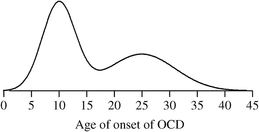
Figure 2.14 The distribution of the age of onset of obsessive compulsive disorder.

The mean value of the age of onset for OCD is µ = 16.2, which is not representative of a typical value in either subpopulation. OCD has two clinical diagnoses, Child Onset OCD and Adult Onset OCD, and the mean values of these subpopulations are μC=10.3 and μA=25, respectively, and clearly, the subpopulation mean values provide more information about their typical values than does the overall mean. The distributions of the Child Onset OCD and Adult Onset OCD are given in Figure 2.15.

Figure 2.15 The distributions of the age of onset of Child Onset and Adult Onset OCD.

Finally, for distributions with extremely long tails, another parameter that can be used to measure the center of the population is the geometric mean . The geometric mean is always less than or equal to the mean ( µ ) and is not as sensitive to the extreme values in the population as the mean is. The geometric mean will be denoted by GM and is defined as

where N is the number of units in the population. That is,

where the X values for the N units in the population are X1,X2,X3,…,XN.

Example 2.16

The distribution given below has a long tail to the right.

In a previous example, µ was computed to be 79.63. The geometric mean for this population is

Thus, even though there is an extremely large and atypical value in this population, the geometric mean is not sensitive to this value and is a more reasonable parameter for representing the typical value in this population. In fact, the geometric mean and median are very close for this population with GM = 29.4 and μ~=28.

While the mean, median, and mode of a population describe the typical values in the population, these parameters do not describe how the population is spread over its range of values. For example, Figure 2.16 shows two populations that have the same mean, median, and mode but different spreads.

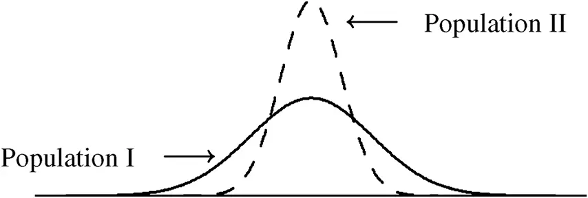
Figure 2.16 Two different populations having the same mean, median, and mode.