Stephen Rolt - Optical Engineering Science

(5.14)

Following this general discussion about the useful properties of orthonormal functions, we can move on to a description of the Zernike circle polynomials themselves. They were initially investigated and described by Fritz Zernike in 1934 and are admirably suited to a solution space defined by a circular pupil. We will suppose initially, that the polynomial may be described by a component, R (ρ), that is dependent exclusively upon the normalised pupil radius and a component G (φ) that is dependent upon the polar angle, φ. That is to say:

(5.15)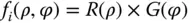

We can make the further assumption that R (ρ) may be represented by a polynomial series in ρ. The form of G (φ) is easy to deduce. For physically realistic solutions, G (φ) must repeat identically every 2π radians. Therefore G (φ) must be represented by a periodic function of the form:

(5.16)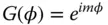

where m is an integer

This part of the Zernike polynomial clearly conforms to the desired form, since not only does it have the desired periodicity, but it also possesses the desired orthogonality. The parameter, m, represents the angular frequency of the polar dependence.

Having dealt with the polar part of the Zernike polynomial, we turn to the radial portion, R (ρ). The radial part of the Zernike polynomial, R (ρ), comprises of a series of polynomials in ρ. The form of these polynomials, R (ρ), depends upon the angular parameter, m , and the maximum radial order of the polynomial, n . Furthermore, considerations of symmetry dictate that the Zernike polynomials must either be wholly symmetric or anti-symmetric about the centre. That is to say, the operation r → − r is equivalent to φ → φ + π. For the Zernike polynomial to be equivalent for both (identical) transformations, for even values of m, only even polynomials terms can be accepted for R (ρ). Similarly, exclusively odd polynomial terms are associated with odd values of m.

Overall, the entirety of the set of Zernike polynomials are continuous and may be represented in powers of P xand P yor ρcos(φ) and ρsin(φ). It is not possible to construct trigonometric expressions of order, m , i.e. cos(mφ) and ρsin(mφ) where the order of the corresponding polynomial is less than m. Therefore, the polynomial, R(ρ), cannot contain terms in ρ that are of lower order than the angular parameter, m.

To describe each polynomial, R (ρ), it is customary to define it in terms of the maximum order of the polynomial, n , and the angular parameter, m . For all values of m (and n ), the polynomial, R (ρ), may be expressed as per Eq. (5.17).

(5.17)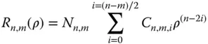

C n,m,i represents the value of a specific coefficient

The parameter, N n,m, is a normalisation factor. Of course, any arbitrary scaling factor may be applied to the coefficients, C n,m,i, provided it is compensated by the normalisation factor. By convention, the base polynomial has a value of unity for ρ = 1. Of course, with this in mind, the purpose of the normalisation factor is to ensure that, in all cases, the rms value of the polynomial is normalised to one. It now remains only to calculate the values of the coefficients, C n,m,i. These are determined from the condition of orthogonality which applies separately for R n,m(ρ) and may be set out as follows:

(5.18)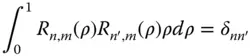

The general formula for the coefficients C n,m,iis set out in Eq. (5.18).

(5.19)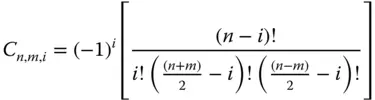

For i = n = 0, the value of the coefficient, C n,m,i, as prescribed for the piston term, is unity. The value of the normalisation factor, N n,m, is given in Eq. (5.20).

(5.20)

More completely we can express the entire polynomial:

(5.21a)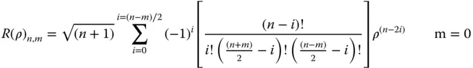

(5.21b)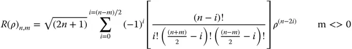

The parameter, m, can take on positive or negative values as can be seen from Eq. (5.16). Of course, Eq. (5.16)gives the complex trigonometric form. However, by convention, negative values for the parameter m are ascribed to terms involving sin(mφ), whilst positive values are ascribed to terms involving cos(mφ).

Zernike polynomials are widely used in the analysis of optical system aberrations. Because of the fundamental nature of these polynomials, all the Gauss-Seidel wavefront aberrations clearly map onto specific Zernike polynomials. For example, spherical aberration has no polar angle dependence, but does have a fourth order dependence upon pupil function. This suggests that this aberration has a radial order, n, of 4 and a polar dependence, m, of zero. Similarly, coma has a radial order of 3 and a polar dependence of one. Table 5.2provides a list of the first 28 Zernike polynomials.

In Table 5.2, each Zernike polynomial has been assigned a unique number. This is the ‘Standard’ numbering convention adopted by the American National Standards Institute, ( ANSI). It has the benefit of following the Born and Wolf notation logically, starting from the piston term which is denominated the zeroth term. If the ANSI number is represented as j, and the Born and Wolf indices as n, m, then the ANSI number may be derived as follows:

(5.22)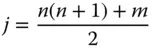

Unfortunately, a variety of different numbering conventions prevail, leading to significant confusion. This will be explored a little later in this chapter. As a consequence of this, the reader is advised to be cautious in applying any single digit numbering convention to Zernike polynomials. By contrast, the n, m numbering convention used by Born and Wolf is unambiguous and should be used where there is any possibility of confusion.