Stephen Rolt - Optical Engineering Science

Adding a conic term to the surface, in addition to defining the curvature of the surface by its base radius, effectively adds an independent term to Eq. (5.9), effectively controlling two polynomial orders in Eq. (5.9). To this extent, adding separate additional second order and fourth order terms to the even asphere expansion in Eq. (5.1)is redundant. From the perspective of controlling third order aberrations, Eq. (5.9)confirms the utility of a conic surface in adding a controlled amount of fourth order optical path difference (OPD) to the system. In fact, the amount of OPD added to the system, to fourth order, is simply given by the change in sag produced by the conic surface multiplied by the difference in refractive indices. If the refractive index of the first medium is n 0, and that of the second medium, n 1, then the change in OPD produced by introducing a conic parameter of k is given by:

(5.10)

Equation (5.10)allows estimation of the spherical aberration produced by a conic surface introduced at the stop position. However, by virtue of the stop shift equations introduced in the previous chapter, providing fourth order sag terms at a surface remote from the stop not only influences spherical aberration, but also the other third order aberrations as well. In principle, therefore, by using aspheric surfaces, it is possible to eliminate all third order aberrations with fewer surfaces that would be possible with using just spherical surfaces alone. In fact, assuming that a system has been designed with zero Petzval curvature, it is only necessary to eliminate spherical aberration, coma, and astigmatism. Therefore, only three surfaces are strictly necessary. This represents a considerable improvement over a system employing only spherical surfaces. Notwithstanding the difficulties in manufacturing aspheric surfaces, some commercial camera systems are designed with this principal in mind.

Having introduced the underlying principles, it must be stated that design using aspheric surfaces is not especially amenable to analytical solution. In principle, of course, Eq. (5.10)could be used together with the relevant stop shift equations to compute analytically all third order aberrations. However, in practice, this is a rather cumbersome procedure and design of such systems proceeds largely by computer optimisation. Nevertheless, a clear understanding of the underlying principles is of invaluable help in the design process. An example, a simple two lens system, employing aspheric surfaces is sketched in Figure 5.3. This lens system replicates the performance of a three lens Cooke triplet with an aperture of f#5 and a field of view of 40°. Figure 5.3is not intended to present a realistic and competitive design, but it merely illustrates the flexibility introduced by the incorporation of aspheric surfaces. In particular, it offers the potential to achieve the same performance with fewer surfaces.

Whilst aspheric components represent a significant enhancement to the toolkit of an optical designer, they represent something of a headache to the component manufacturer. As will be revealed later, in general, aspheric components are more difficult to manufacture and test and hence more costly. As such, their use is restricted to those situations where the advantage provided is especially salient. At the same time, advanced manufacturing techniques have facilitated the production of aspheric surfaces and their application in relatively commonplace designs, such as digital cameras, is becoming a little more widespread. Of course, the presence of conic and aspheric surfaces in large reflecting telescope designs is, by comparison, relatively well established.

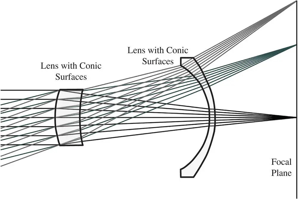
Figure 5.3 Simple two lens system employing aspheric components.

In describing wavefront aberrations at any surface in a system, it is convenient to do so by expressing their value in terms of the two components of normalised pupil functions P xand P y. Where the magnitude of the pupil function is equal to unity, this describes the position of a ray at the edge of the pupil. With this description in mind, we now proceed to describe the normalised pupil position in terms of the polar co-ordinates, ρ and θ. This is illustrated in Figure 5.4.

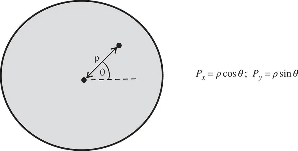
Figure 5.4 Polar pupil coordinates.

The wavefront error across the pupil can now be expressed in terms of ρ and θ. What we are seeking is a set of polynomials that is orthonormal across the circular pupil described. Any continuous function may be represented in terms of this set of polynomials as follows:

(5.11)

The individual polynomials are described by the term f i(ρ,θ), and their magnitude by the coefficient, A i. The property of orthonormalityis significant and may be represented in the following way:

(5.12)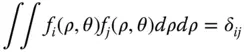

The symbol, δ ijis the Kronecker delta. That is to say, when i and j are identical, i.e. the two polynomials in the integral are identical, then the integral is exactly one. Otherwise, if the two polynomials in the integral are different, then the integral is zero. The first property is that of normality, i.e. the polynomials have been normalised to one and the second is that of orthogonality, hence their designation as an orthonormalpolynomial set.

Equations (5.11)and (5.12)give rise to a number of important properties of these polynomials. Initially we might be presented with a problem as to how to represent a known but arbitrary wavefront error, Φ(ρ,θ) in terms of the orthonormal series presented in Eq. (5.11). For example, this arbitrary wavefront error may have been computed as part of the design and analysis of a complex optical system. The question that remains is how to calculate the individual polynomial coefficients A i. To calculate an individual term, one simply takes the cross integral of the function, Φ(ρ,θ), with respect to an individual polynomial, f i(ρ, θ):

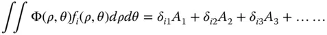
By definition we have:

(5.13)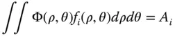

So, any coefficient may be determined from the integral presented in Eq. (5.13). The coefficients, A i, clearly express, in some way, the magnitude of the contribution of each polynomial term to the general wavefront error. In fact, the magnitude of each component, A i, represents the root mean square (rms) contribution of that component. More specifically, the total rms wavefront error is given by the square root of the sum of the squares of the individual coefficients. That this is so is clearly evident from the orthonormal property of the series: