Stephen Rolt - Optical Engineering Science

An air spaced achromatic doublet may be optimised to eliminate both spherical aberration and coma. The fundamental power of the wavefront approach in describing third order aberration is reflected in the ability to calculate the total system aberration as the sum of the aberration of the two lenses. In the thin lens approximation, we may simply use Eqs. (4.30a)and (4.30b)to express the spherical aberration and coma contribution for each lens element. We simply ascribe a variableshape parameter, s 1and s 2to each of the two lenses. The two conjugate parameters are fixed. In the particular case of a doublet designed for the infinite conjugate, the conjugate parameter for the first lens, t 1, is −1. In the case of the second lens, the conjugate parameter, t 2, is determined by the relative focal lengths of the two lenses and thus fixed by the ratio of the two Abbe numbers and, from Eq. (4.52), we get:

(4.53)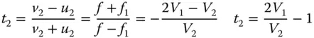

Without going through the algebra in detail, it is clear that having determined both t 1and t 2, Eqs. (4.30a)and (4.30b)give us two expressions solely in terms of s 1and s 2. These expressions for the spherical aberration and coma must be set to zero and can be solved for both s 1and s 2. The important point to note about this procedure is that because Eq. 4.30acontains terms that are quadratic in shape factor, this is also reflected in the final solution. Therefore, in general, we might expect to find two solutions to the equation and this, in general, is true.

At this point we illustrate the design of an air spaced achromat by looking more closely at the previous example where we analysed a 200 mm achromat design. We are to design an achromat with a focal length of 200 mm working at the infinite conjugate, using SCHOTT N-BK7 and SCHOTT SF2 as the two glasses, with the less dispersive N-BK7 used as the positive ‘crown’ element. Again, the Abbe numbers for these glasses are 64.17 and 33.85 respectively and the n dvalues (refractive index at 589.6 nm) 1.5168 and 1.647 69. From the previous example, we know that focal lengths of the two lenses are:

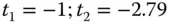
The two conjugate parameters are straightforward to determine. The first conjugate parameter, t 1, is naturally −1. Eq. (4.53)can be used to determine the second conjugate parameter, t 2. This gives:

We now substitute the conjugate parameter values together with the refractive index values (ND) into Eq. (4.30a). We sum the contributions of the two lenses giving the total spherical aberration which we set to zero. Calculating all coefficients we get a quadratic equation in terms of the two shape factors, s 1and s 2.

(4.54)

We now repeat the same process for Eq. (4.30b), setting the total system coma to zero. This time we get a linear equation involving s 1and s 2.

(4.55)

Substituting Eq. (4.55)into Eq. (4.54)gives the desired quadratic equation:

(4.56)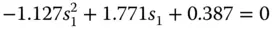

There are, of course, two sets of solutions to Eq. (4.56), with the following values:

Solution 1: s1 = −0.194; s2 = 1.823

Solution 2: s1 = 3.198; s2 = 2.929

There now remains the question as to which of these two solutions to select. Using Eq. (4.29)to calculate the individual radii of curvature from the lens shapes and focal length we get:

Solution 1: R1 = 121.25 mm; R2 = −81.78 mm; R3−81.29 mm; R4 = −281.88 mm

Solution 2: R1 = 23.26 mm; R2 = 44.43 mm; R3−58.91 mm; R4 = −119.68 mm

The radii R 1and R 2refer to the first and second surfaces of lens 1 and R 3and R 4to the first and second surfaces of lens 2. It is clear that the first solution contains less steeply curved surfaces and is likely to be the better solution, particularly for relatively large apertures. In the case of the second solution, whilst the solution to the third order equations eliminates third order spherical aberration and coma, higher order aberrations are likely to be enhanced.

The first solution to this problem comes under the generic label of the Fraunhofer doublet, whereas the second is referred to as a Gauss doublet. It should be noted that for the Fraunhofer solution, R 2and R 3are almost identical. This means that should we constrain the two surfaces to have the same curvature (in the case of a cemented doublet) and just optimise for spherical aberration, then the solution will be close to that of the ideal aplanatic lens. To do this, we would simply use Eq. 4.29, forcing R 2and R 3to be equal and to replace Eq. 4.55constraining the total coma, providing an alternative relation between s 1and s 2. However, the fact that the cemented doublet is close to fulfilling the zero spherical aberration and coma condition further illustrates the usefulness of this simple component.

The analysis presented applies only strictly in the thin lens approximation. In practice, optimisation of a doublet such as presented in the previous example would be accomplished with the aid of ray tracing software. However, the insights gained by this exercise are particularly important. For instance, in carrying out a computer-based optimisation, it is critically important to understand that two solutions exist. Furthermore, in setting up a computer-based optimisation, an exercise, such as this, provides a useful ‘starting point’.

The previous analysis of the achromatic doublet provides a means of ameliorating the impact of glass dispersion and to provide correction at two wavelengths. In the case of the standard visible achromat, correction is provided at the F and C wavelengths, the two hydrogen lines at 486.1 and 656.3 nm. Unfortunately, however, this does not guarantee correction at other, intermediate wavelengths. If one views dispersion of optical materials as a ‘small signal’ problem, and that any difference in refractive index is small across the region of interest, then correction of the chromatic focal shift with a doublet may be regarded as a ‘linear process’. That is to say we might approximate the dispersion of an optical material by some pseudo-linear function of wavelength, ignoring higher order terms. However, by ignoring these higher order terms, some residual chromatic aberration remains. This effect is referred to as secondary colour.The effect is illustrated schematically in Figure 4.26which shows the shift in focus as a function of wavelength.

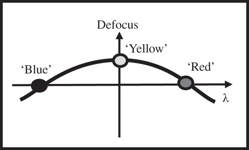
Figure 4.26 Secondary colour.